The slides used in this video are shown below:
Slide 1
Welcome to the training course on IBM Scalable Architecture for Financial Reporting, or SAFR. This is Module 15, Lookups using Constants and Symbolics
Slide 2
Upon completion of this module, you should be able to:
- Read a Logic Table and Trace with constants and symbolics in lookup key fields
- Explain the Function Codes used in the example
- Debug lookups with symbolics
- Use selected Logic Table Trace Parameters
Slide 3
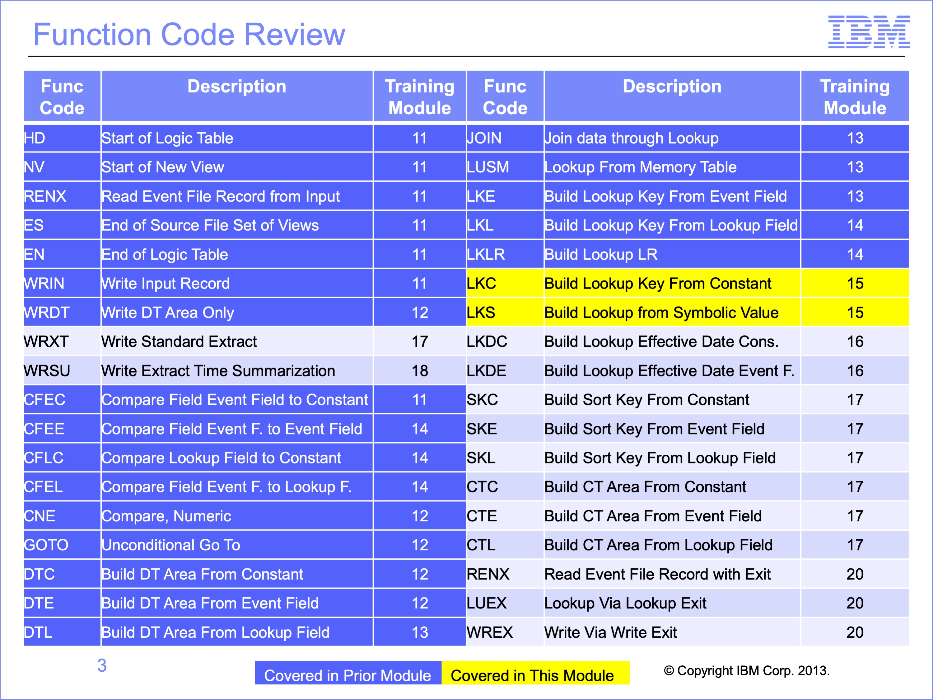
The prior modules covered the function codes highlighted in blue. Those to be covered in this module are highlighted in yellow.
Slide 4
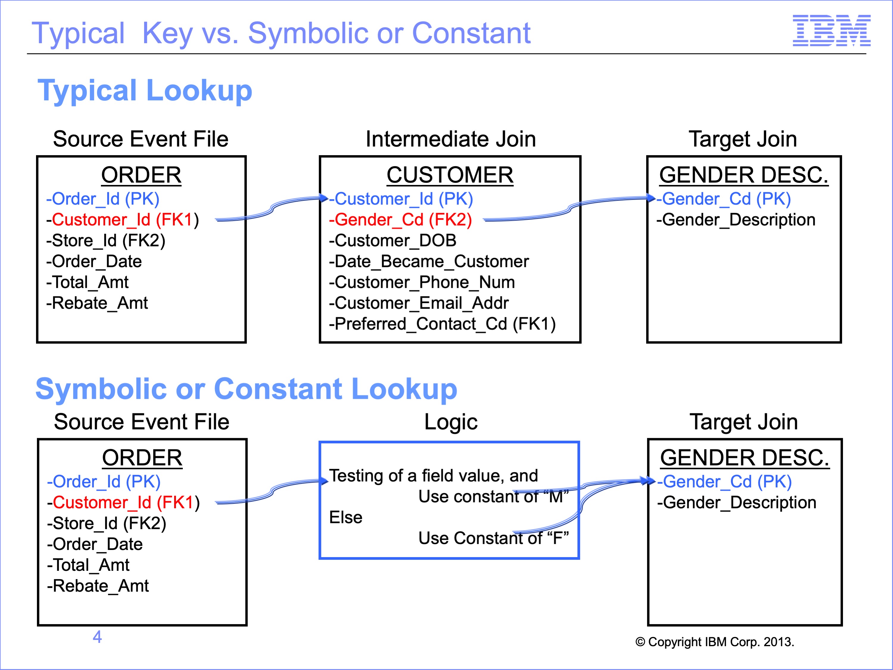
Most lookups use key values provided by other LRs, starting with the Source Event LR, and values in the source and target fields are the same. In some cases data values in the input file and those in the reference file cannot be simply matched for a join. Yet through use of logic, the relationship might be programmed. The person building the join and view must know the data to properly use these types of joins.
If in our example, we did not have a Customer Table to give us the customer code, the value to find the Gender would need to be provided through the view in some way.
This can be accomplished in 2 ways:
- A Constant can be added to the Lookup Path when defined. The view cannot change the constant
- A Symbolic can be defined in the Lookup Path. The value of the symbolic is assigned in the view
In either case, the value remains the same throughout the processing of the view.
Slide 5

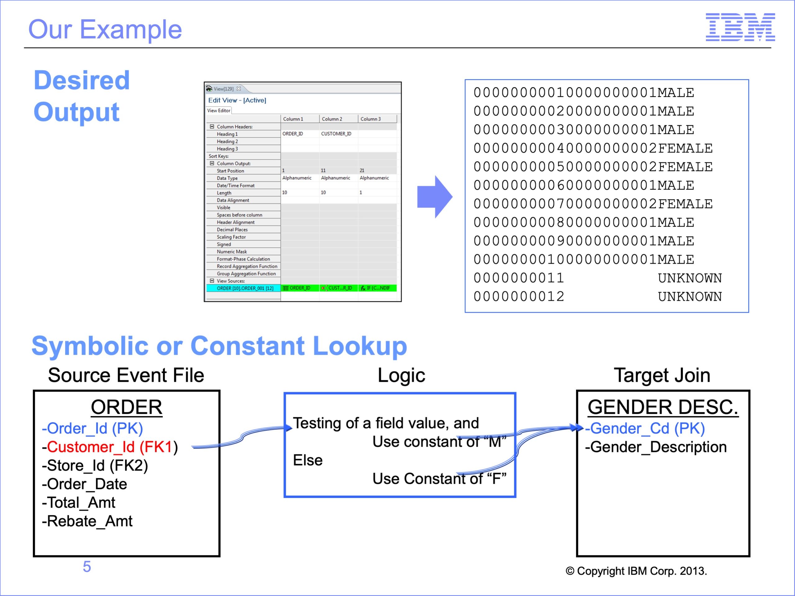
We’ll use a similar example to the prior module, where we wish to output the Order ID, Customer ID and the Customer Gender Code. In our example, we won’t change either the input or output data, so a typical join could be used. We’ll show that a constant could be if either the source field or the target field were different values
Slide 6
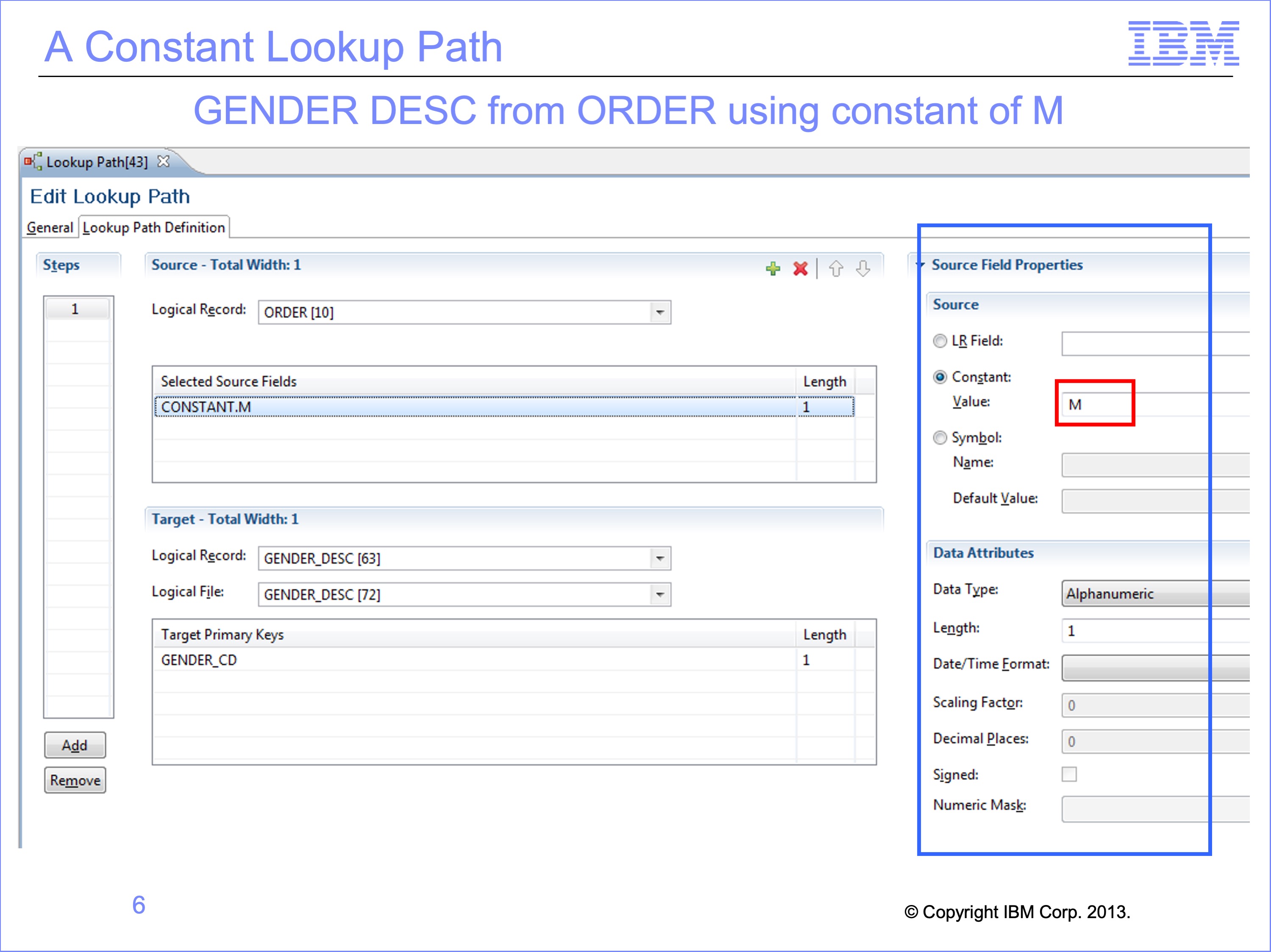
Both types of joins still require the source and target logical records to be specified, even when no fields from the source are used in the search. Constants and symbolics can be used in combination with fields to perform a join, or they can be the only value to search the target reference file. They can also be used in any step of a join.
A Constant can be used if the same value should be used in every search of the reference file. The value to be used in the search for a matching record is placed directly in the Look-up Path definition. The data type format must also be specified correctly to match the key data of the target reference file.
For our example we have defined this lookup path to use a constant of “M” for the Customer Code key. We will also use another lookup path with a constant of “F”, which is not shown.
Slide 7
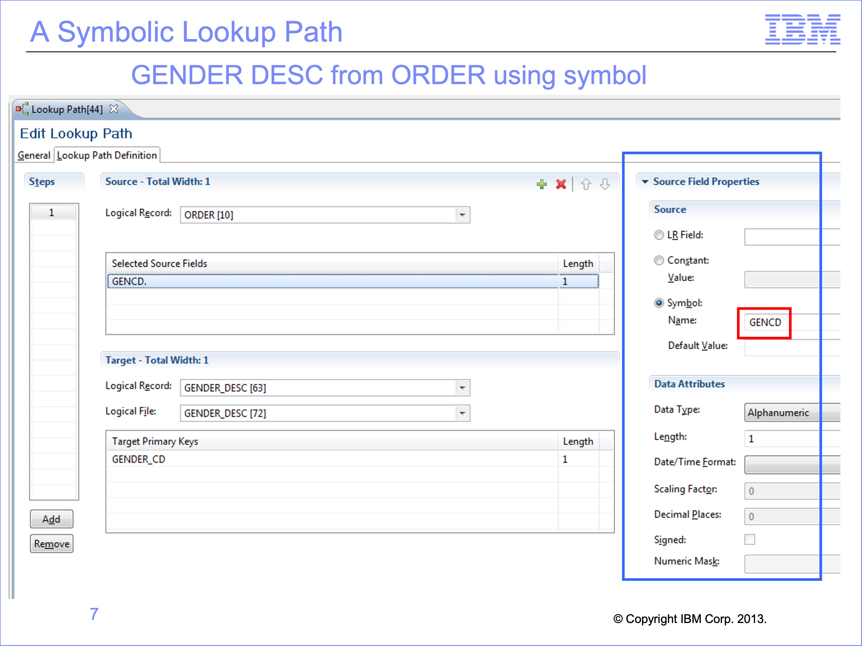
A symbolic join is also defined in the lookup path. But unlike the constant join, the value to be used in the search is not yet defined. Rather, the symbolic is a key word that will be used in the view to assign what value should be used to search the target reference table. In other words, the symbolic is a variable that is resolved using logic text in the view.
Constants, symbolics and LR fields can be used together in the same join in any order or any combination.
In our example, we’ve defined a symbolic of GENCD for the Gender Code which we will assign in Logic Text.
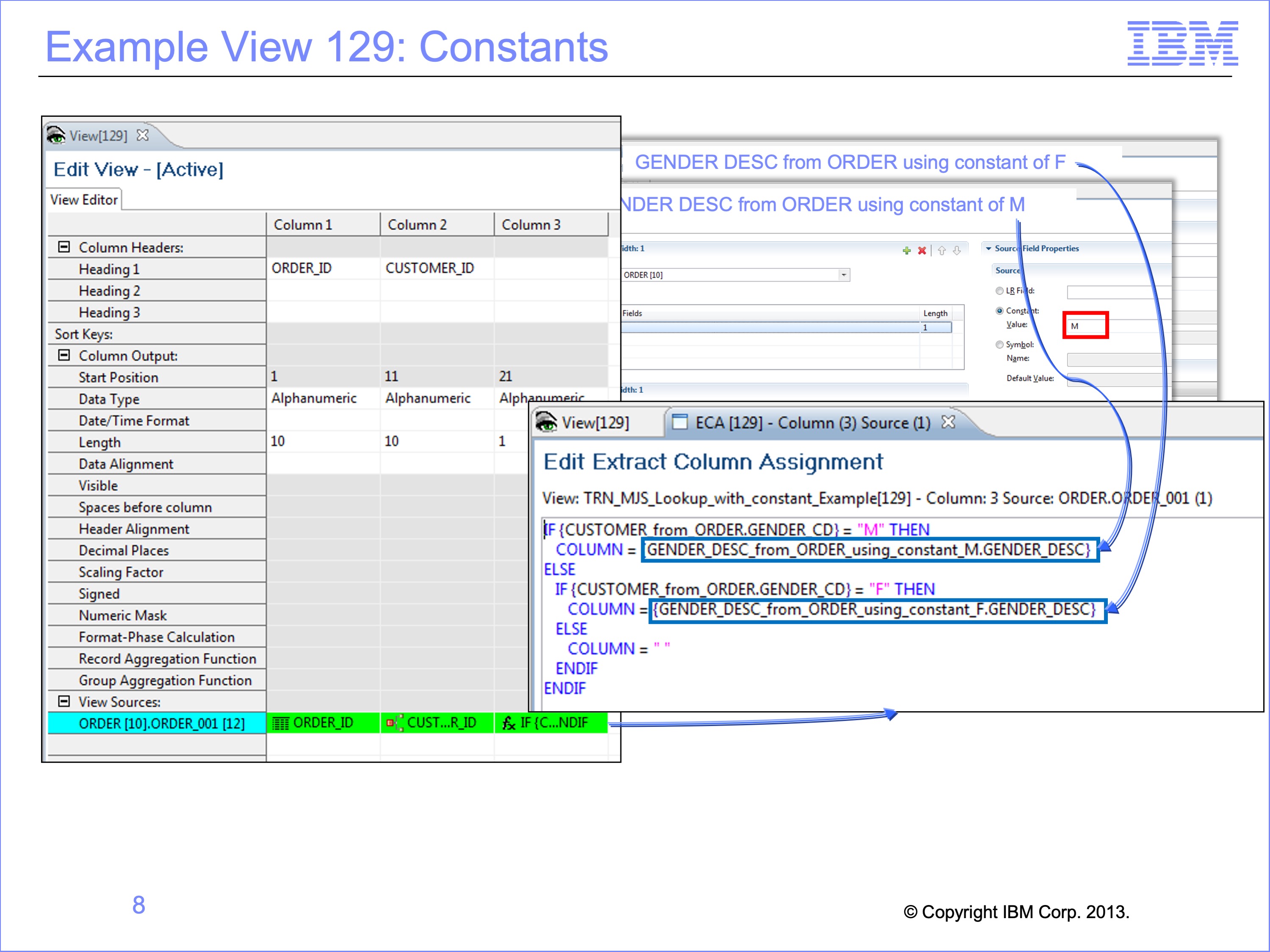
Slide 8
Lookup paths that contain constants or symbolics are used like any other paths in views. In both our example views we will use them in logic text.
We’ll use view 129 to demonstrate how paths with embedded constants operate. In Column 3 of this view, our logic text will first look up to the Customer table using the Customer ID to find the Gender Code of either “M” or “F”. Instead of using this as the key to the Gender Description table, we will use our new constant paths.
Slide 9
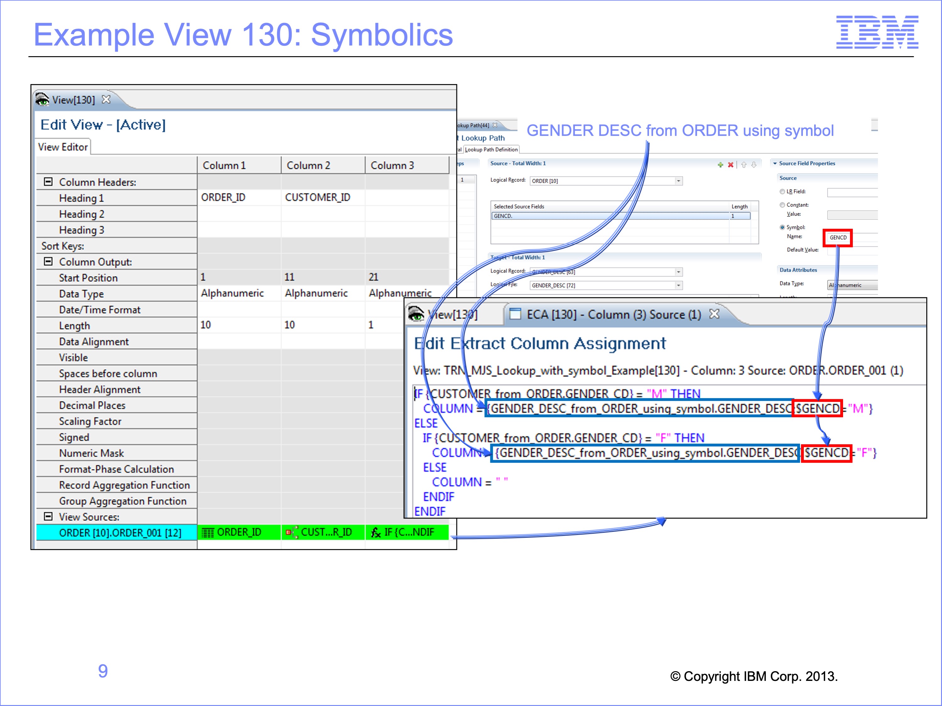
Symbolic views require logic text in order to assign the symbolic value. The symbol (or variable) assigned in the path is assigned a value within the logic. This is done by using the path name, followed by a semicolon, a dollar sign and the symbol name, and equal sign and then an assigned value as a constant. Multiple symbolics can be assigned values one right after the others.
Our example view 130 shows how symbolics work. As shown, the path name is used, followed by a semicolon, a dollar sign and the symbolic name “$GENCD”, an equal sign and a constant. Notice that instead of requiring two paths on the prior view, one for “M” and the other for “F”, we now are able to use a single path for both conditions.
Slide 10
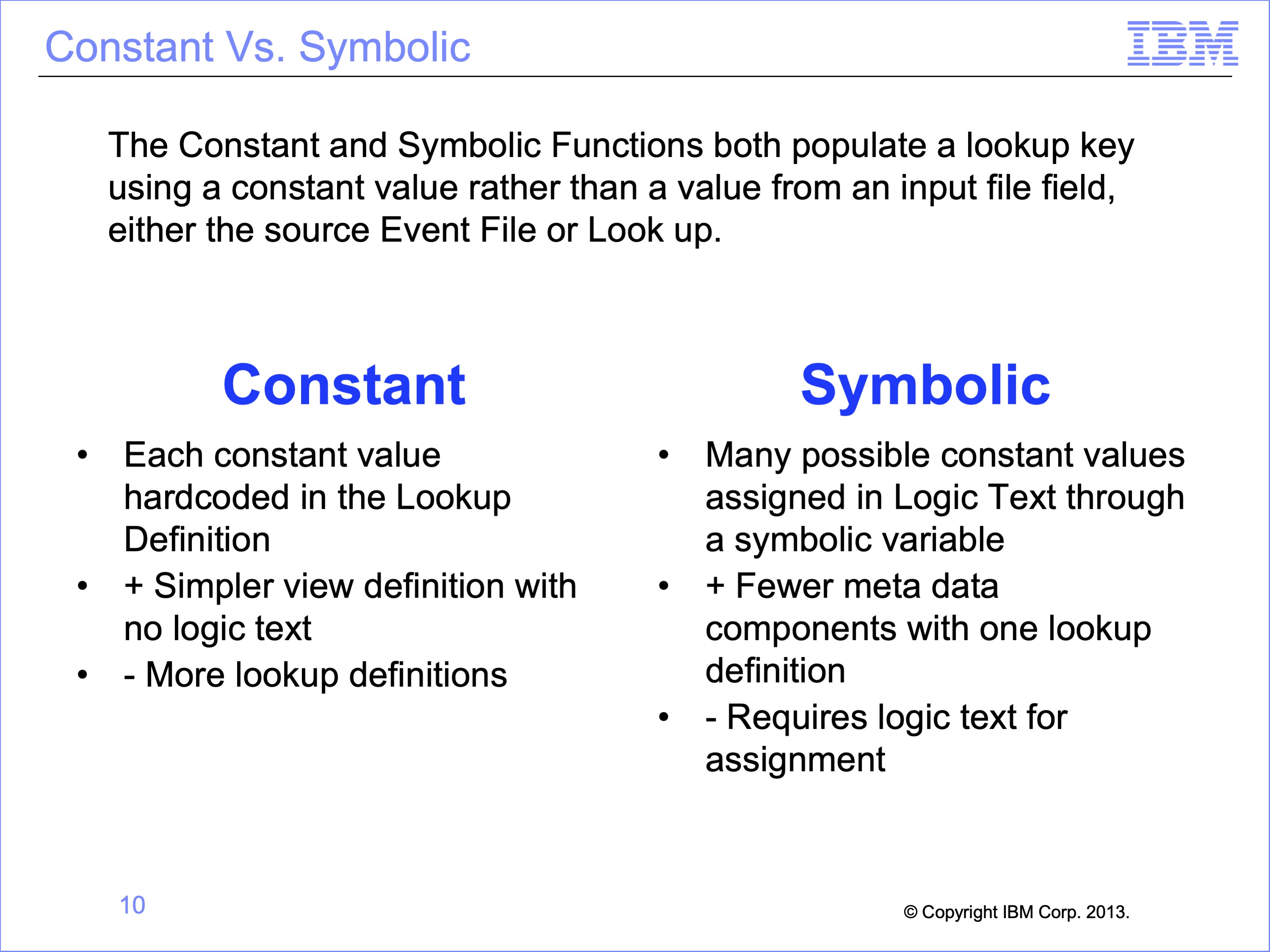
The Constant and Symbolic Functions both populate a lookup key using a constant value rather than a value from an input file field, either the source Event File or Look up.
A Constant value is hardcoded in the Lookup Definition, which in turn simplifies view definition with no logic text, but requires more lookup definitions.
A Symbolic allows many possible constant values assigned in Logic Text through a symbolic variable, which means fewer total components with one lookup definition, but each use requires logic text for assignment
Slide 11
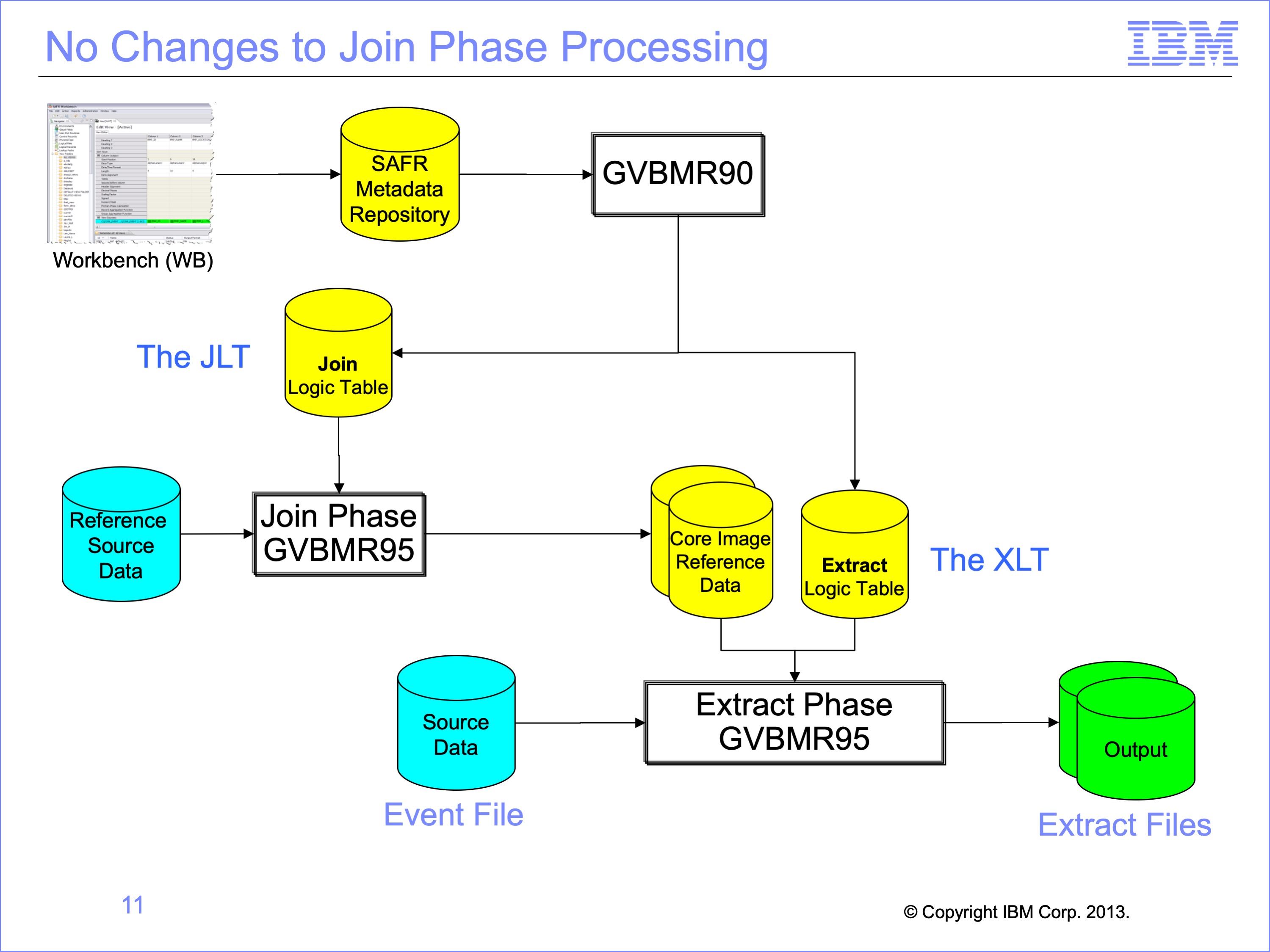
Constant and Symbolic joins do not affect the JLT process in any way. Core image reference files are produced as they would be for any other join. Constant and symbolic joins only affect the XLT, and as we will see, in very small ways.
Slide 12
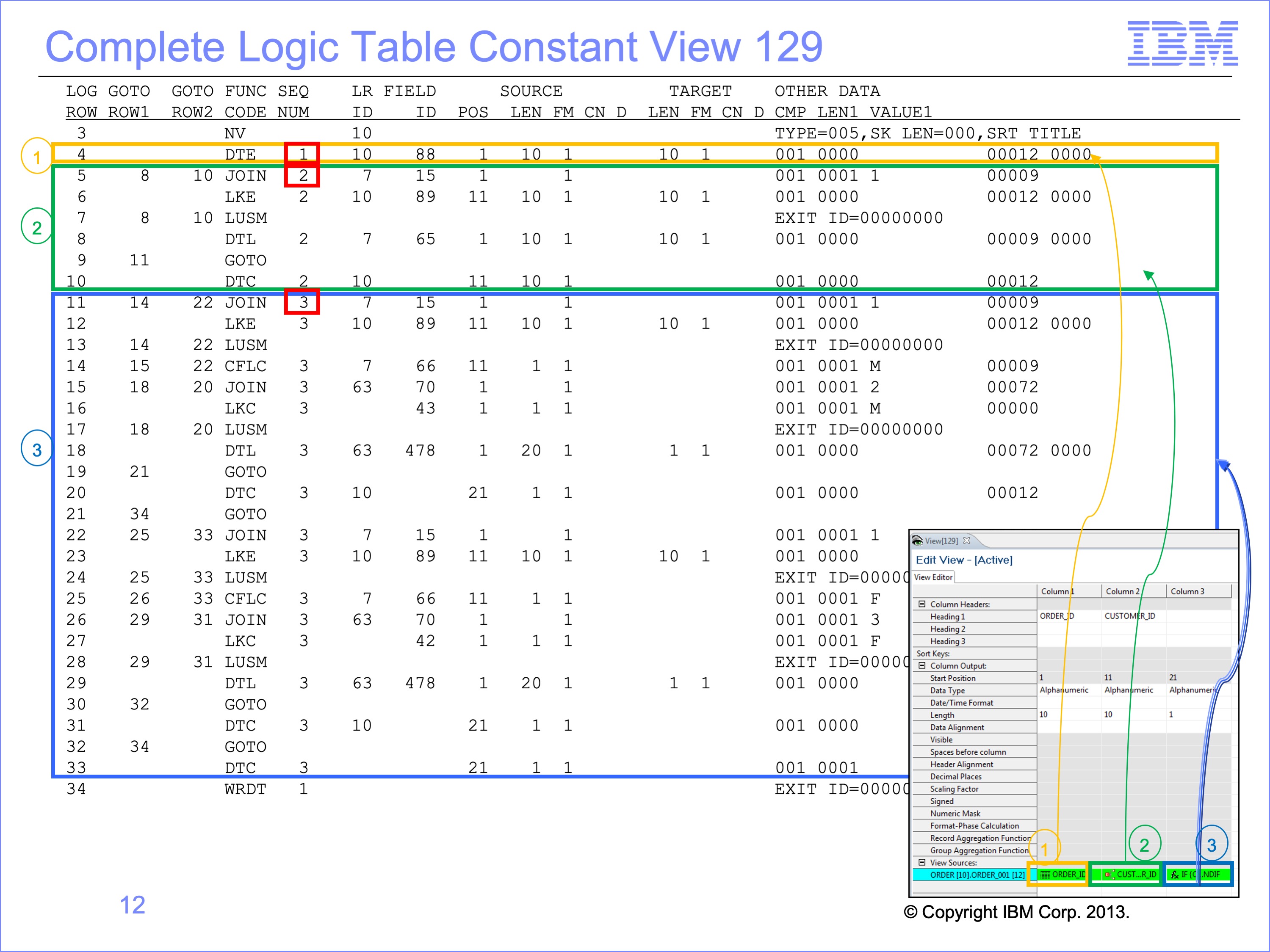
This is the complete logic table for the constant view, view 129. The view has no extract record filtering. Thus it is composed almost entirely of column dependent logic table rows. Column 1 requires one row, a DTE to populate the Order ID. Column 2 requires logic table rows 5 – 10, a join to the Customer Table to obtain the Customer ID. Column 3 requires rows 11 through 33 to populate the Customer Gender Code using our lookup paths with embedded constants.
Slide 13
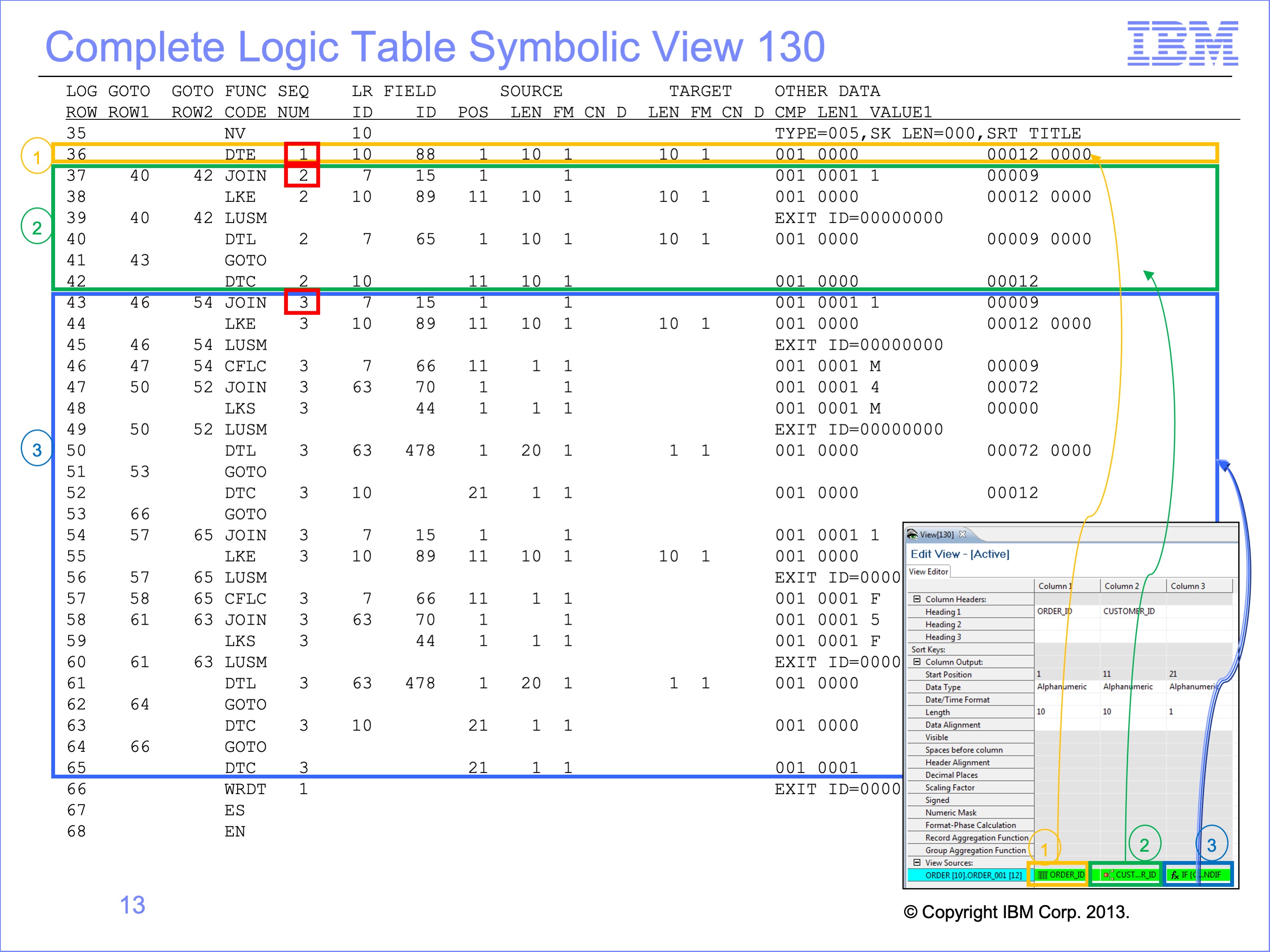
This is the complete logic table for the symbolic view, view 130. It has by and large the same structure as the constant view. One difference is the LT row numbers differ because view 130 is executed in the same Performance Engine run as view 129. Its LT rows are therefore after those of view 129.
We’ll focus our attention in this module on Column 3, and compare and contrast the differences between these two views and their different paths. For this logic table row comparison, we’ll change view 130 row numbers to be consistent with view 129.
Slide 14
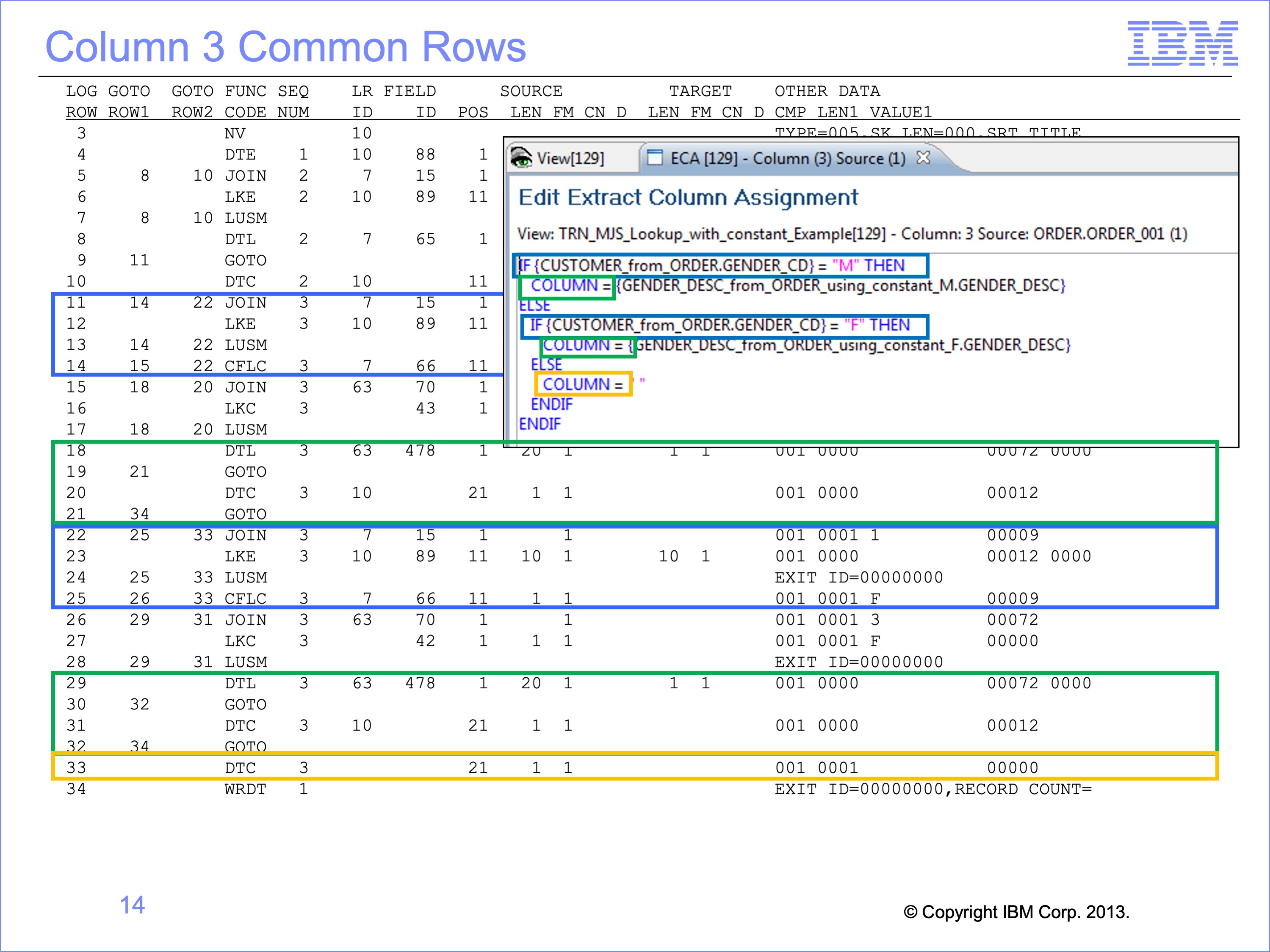
Inside column 3 logic, both views perform the same lookup to the Customer file to determine the Gender of the Customer. The first test is for “M”, and a second test for “F”. Both views also have the same patterned DTL and DTC functions for populating the column based upon lookup results. When we eliminate all these rows of the logic table for our comparison, we are down to very few rows to analyze.
Slide 15
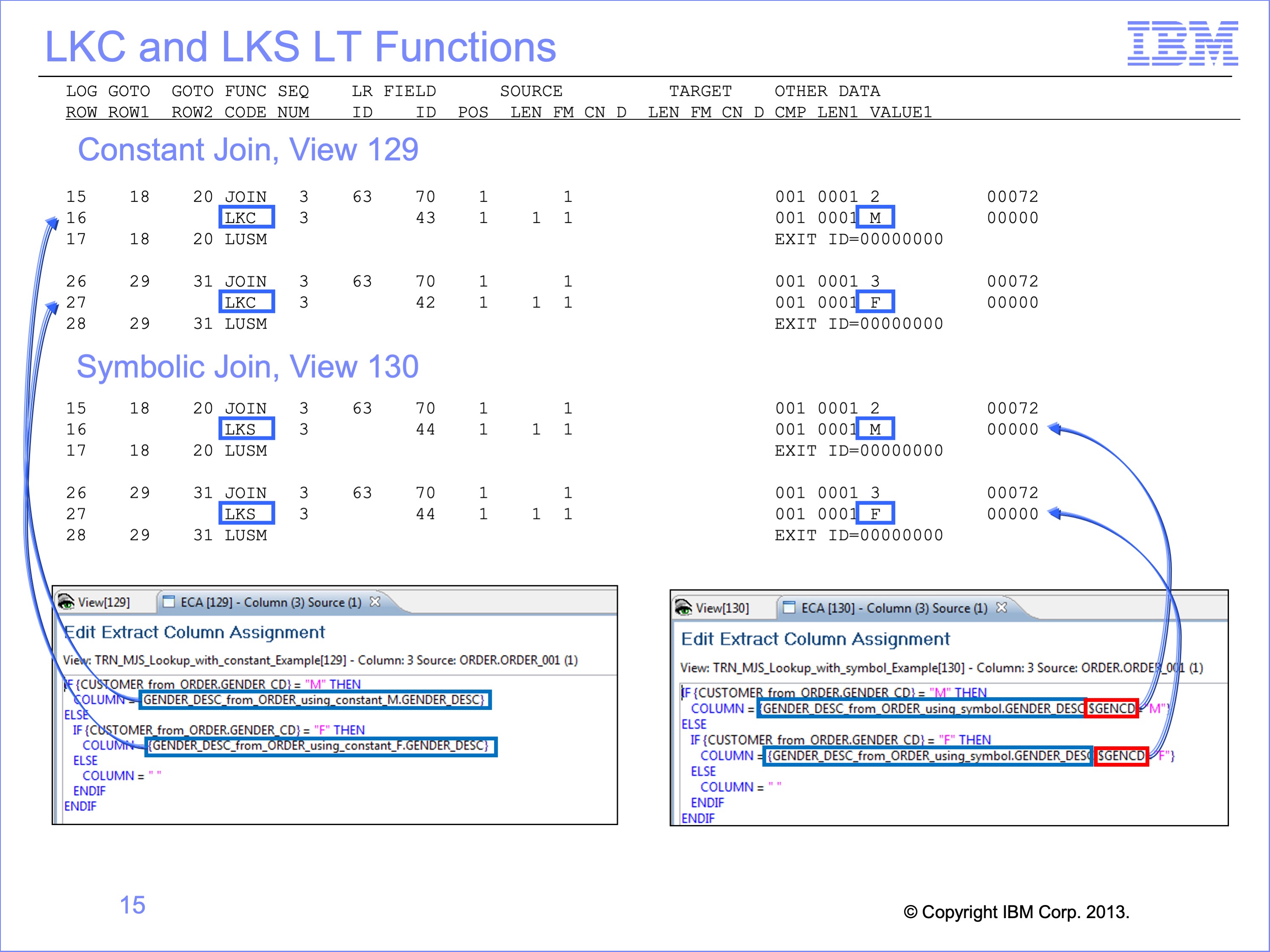
Lookup paths containing Constants have an LKC Lookup Constant Logic Table Function. This function code, similar to an LKE and LKL builds a lookup key value to be used when searching a core image file. The LKC simply places a constant in the key.
In our view 129 example two LKC’s are used, one each to satisfy the join required by the COLUMN = keyword. One assigns a value of “M” to the key, the other a value of “F”.
Symbolic paths contain LKS Lookup Symbolic Logic Table Functions. This function performs the same operation as the LKC, placing a constant in the lookup key before searching a core image file.
Example view 130 similarly has two LKS functions, one assigning a “M” and the other assigning an “F” before the respective LUSM functions.
Slide 16
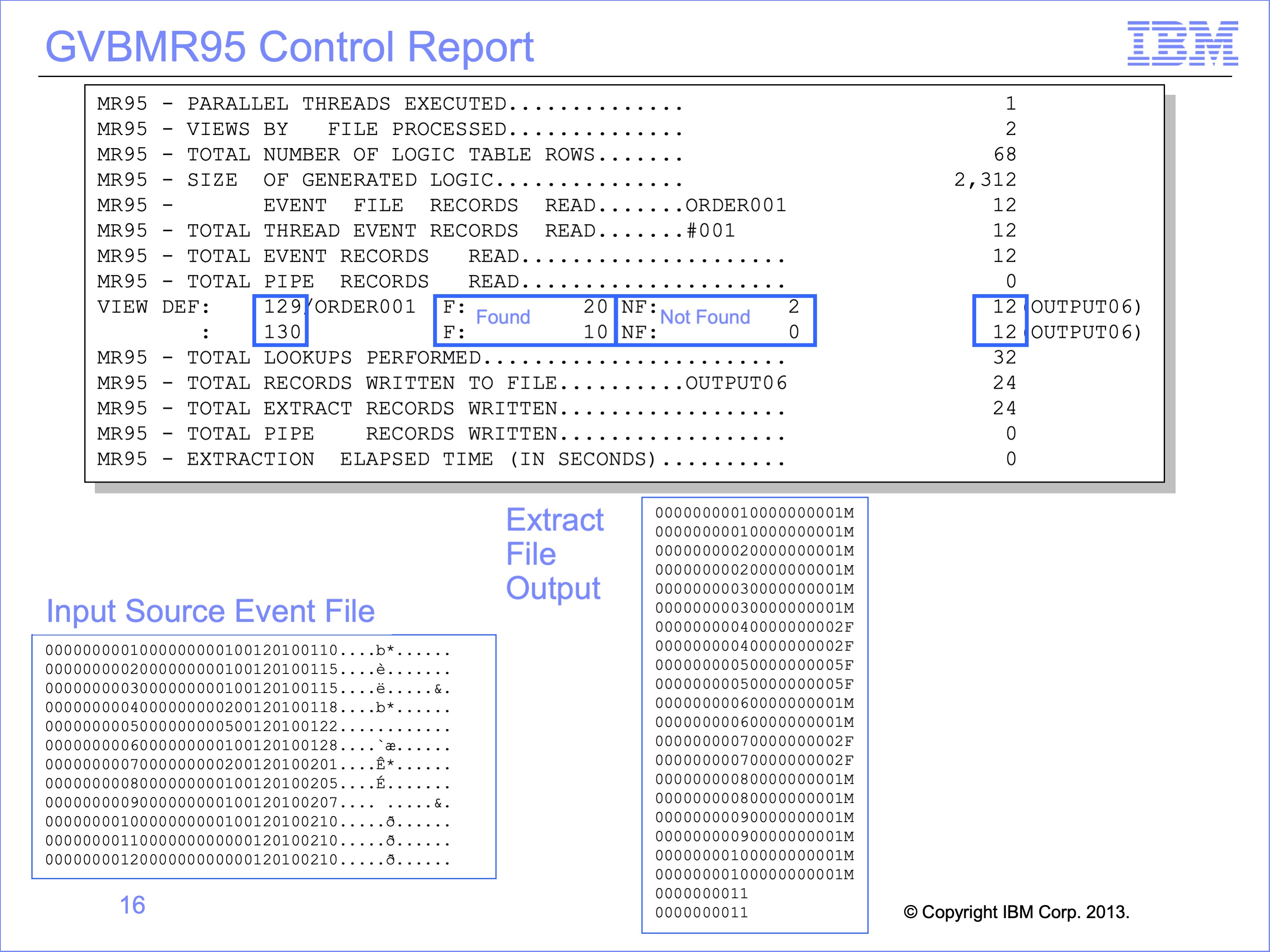
Before examining the trace results, let’s look at the Extract Engine GVBMR95 control report to see the results of running these views.
Both views have written 12 output records. But the found and not found counts are not the same. Remember that Found and Not Found counts are the results of LUSM functions, and join optimization might simple cause view 130 to perform fewer of these functions.
Both views wrote their output to the same output file, DD Name OUTPUT06. Thus records from view 129 are interspersed with records from view 130. If we examine the file carefully, it appears that each record is basically duplicated, which is what we would expect because the views create effectively the same output in slightly different ways. And we can see that there appears to be two records, one for each view, which does not have a customer ID or Gender Code.
Lastly, because we were looking up to the Gender Description table, we would have expected to see “MALE” and “FEMALE” on the records, not the “M” and “F” displayed. Let’s use the Logic Table Trace to examine these potential issues.
Slide 17
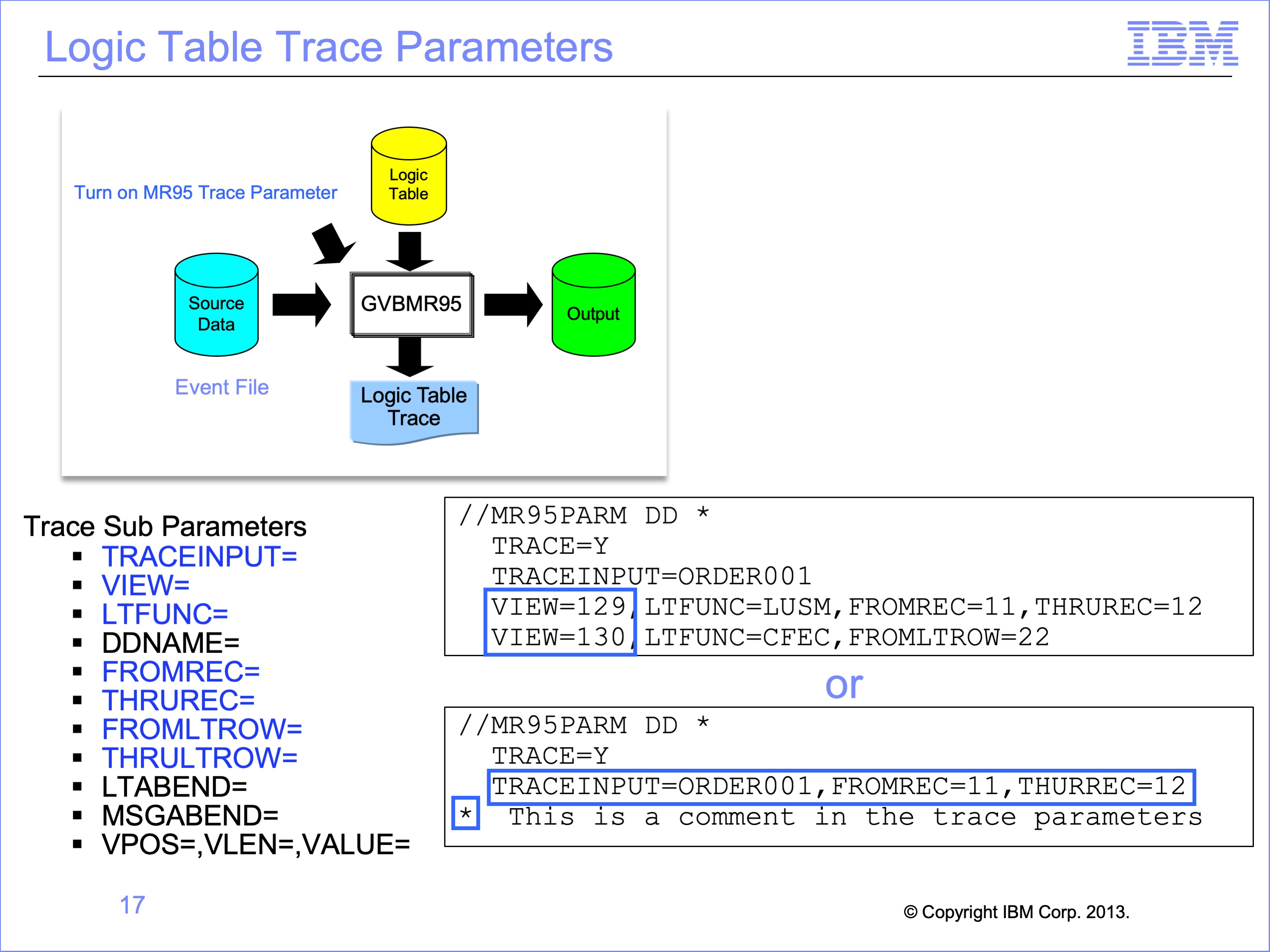
In the Introduction to Trace Facilities we briefly discussed the additional parameters available to control what is traced. We’ll use those parameters highlighted in blue to investigate our view results.
Although multiple trace parameters can be used at one time only one global parameter is permitted. The global parameter is the one with no VIEW keyword on it. Besides the one global parameter, all trace parameter rows require a VIEW parameter or they will be ignored in trace processing.
In the top example, the global parameter TRACEINPUT is used, and then two views each have individual trace parameters.
In the bottom example, only a global parameter is used which will affect all rows in the logic table for all views.
Note that an asterisk in the first position of the MR95PARMs marks a comment, which can be useful for saving prior trace parameters.
Slide 18
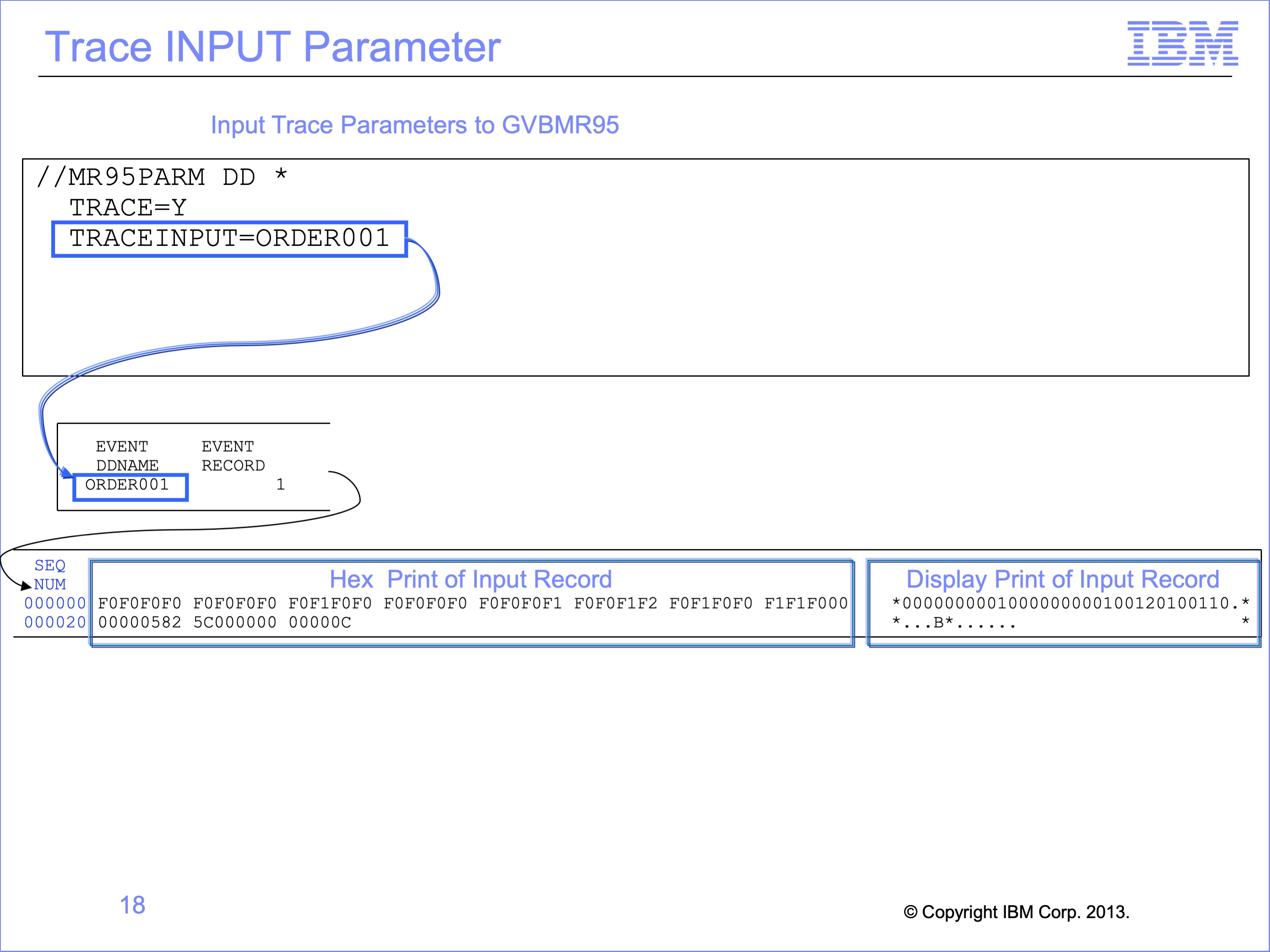
The TRACEINPUT parameter causes GVBMR95 to print the source Event File record. The parameter is followed by the DD Name of the Event File to be traced. In the Trace output the DD name is followed by the record number being printed.
The headings for the Trace Report have been removed in this example to make the printout more clear, and because of the report width is it shown in two parts.
The input record is printed in two forms, as HEX characters which can allow viewing of things like packed and binary numbers, and as display characters which are easier for reading text.
The SEQ NUM column before the Hex characters contains an index to the character positions of the printed hex record. In this example, the first hex value of “F0F0F0F0” begins at offset “000000”. On the next row the hex value of “00000582” begins at offset 000020 from the start of the record. Note that a hex 20 is a decimal 32 bytes from the beginning of the record.
Slide 19
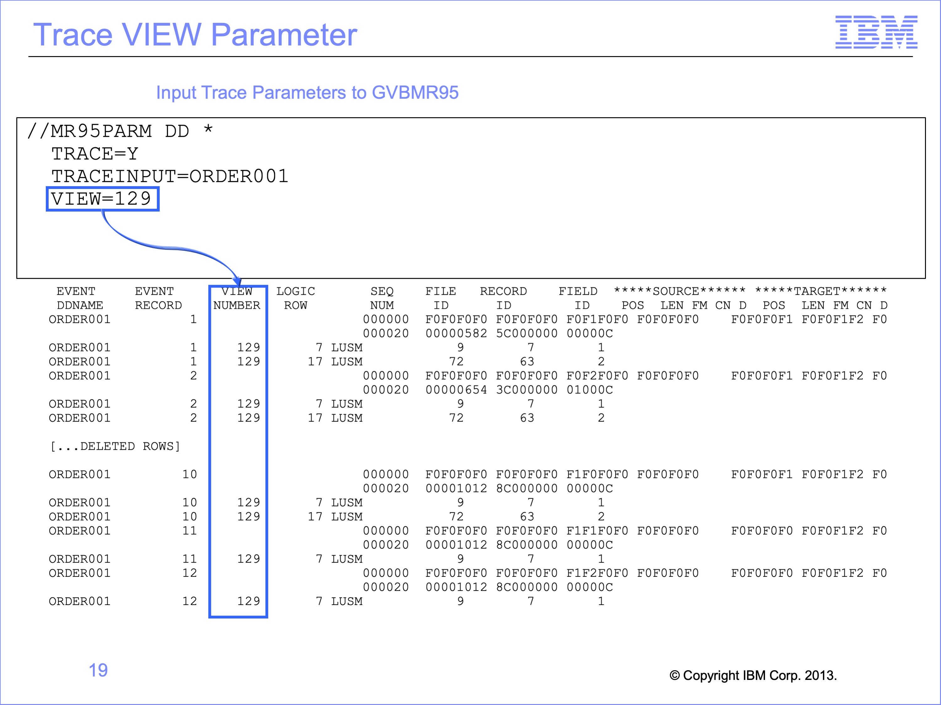
The Trace View Parameter indicates which view should be traced. In this example, only view 129 will be traced. Notice that the trace output does not include any trace rows from view 130 even though it was contained in the same logic table and was processed by the Extract Engine at the same time. This is a simple way of reducing the trace output to a single view of interest.
Slide 20
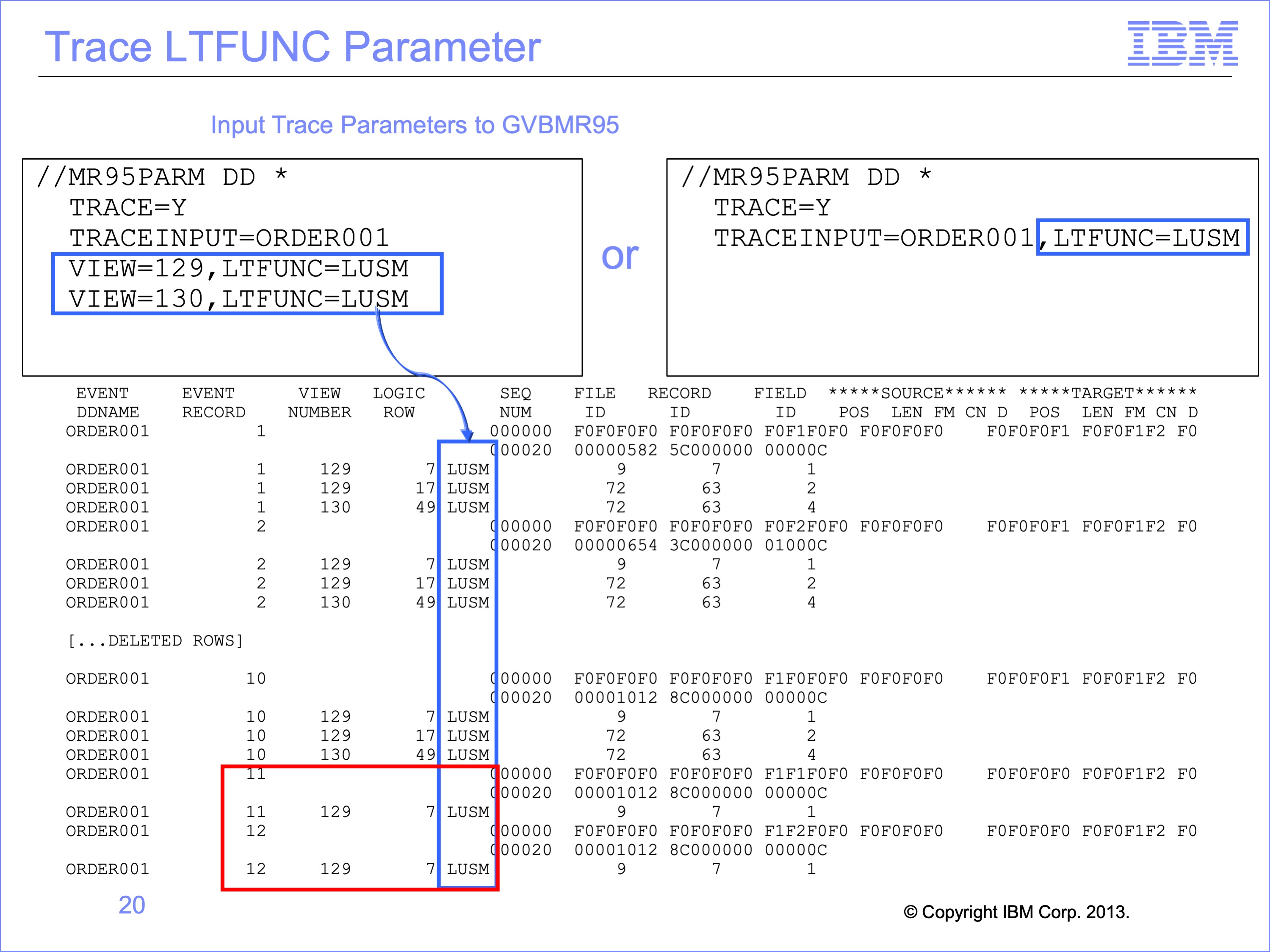
Another useful keyword is the LTFUNC parameter.
Multiple VIEW parameters can be used at the same time. In this example, all LUSM functions for both views are shown. Because we are looking for the same function codes in all the views in the logic table, the same thing could have been accomplished by coding the LTFUNC parameter on the Global Trace Parameter line.
Notice on this trace that for the last two records in the input file, records 11 and 12, only view 129 performed any LUSM functions. This might explain the differences between Found and Not Found lookup on the GVBMR95 Control report.
Slide 21
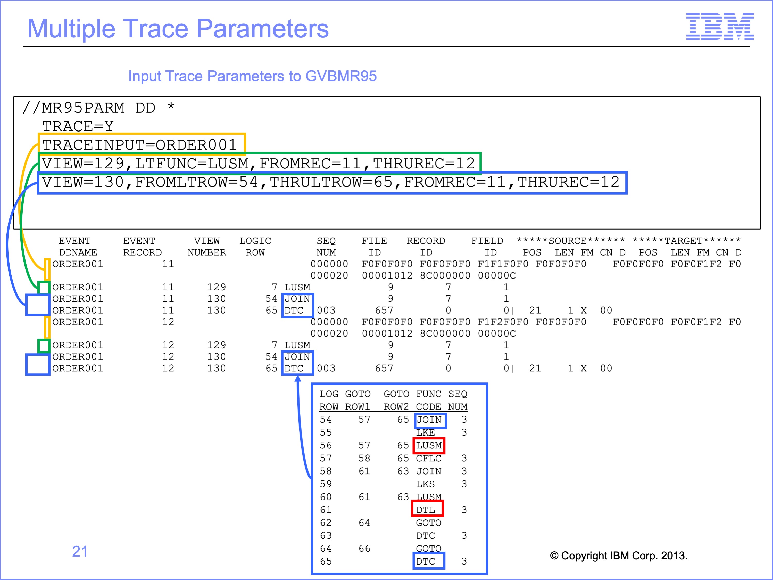
Multiple trace parameters can be used together with different sub parameters as well.
- In this example the orange boxes highlight the Global parameter request for a print of the input record from the ORDER001 DD Name
- The green boxes show the VIEW=129 parameters print only the LUSM function code rows on input records 11 and 12 and the output.
- The blue boxes highlight the VIEW=130 parameters requesting the trace to print all LT function codes from Logic Table Rows 54 to 65, on input records 11 and 12.
The output from these last set of parameters shows that only the JOIN function code of LT Row 54 and the DTC of LT Row 65 were executed. The LUSM and the DTL function codes allow in this section of the Logic Table were not executed. Thus we can confirm that because the LUSM was not executed the Found and Not Found counts between view 129 and view 130 should be different.
Slide 22
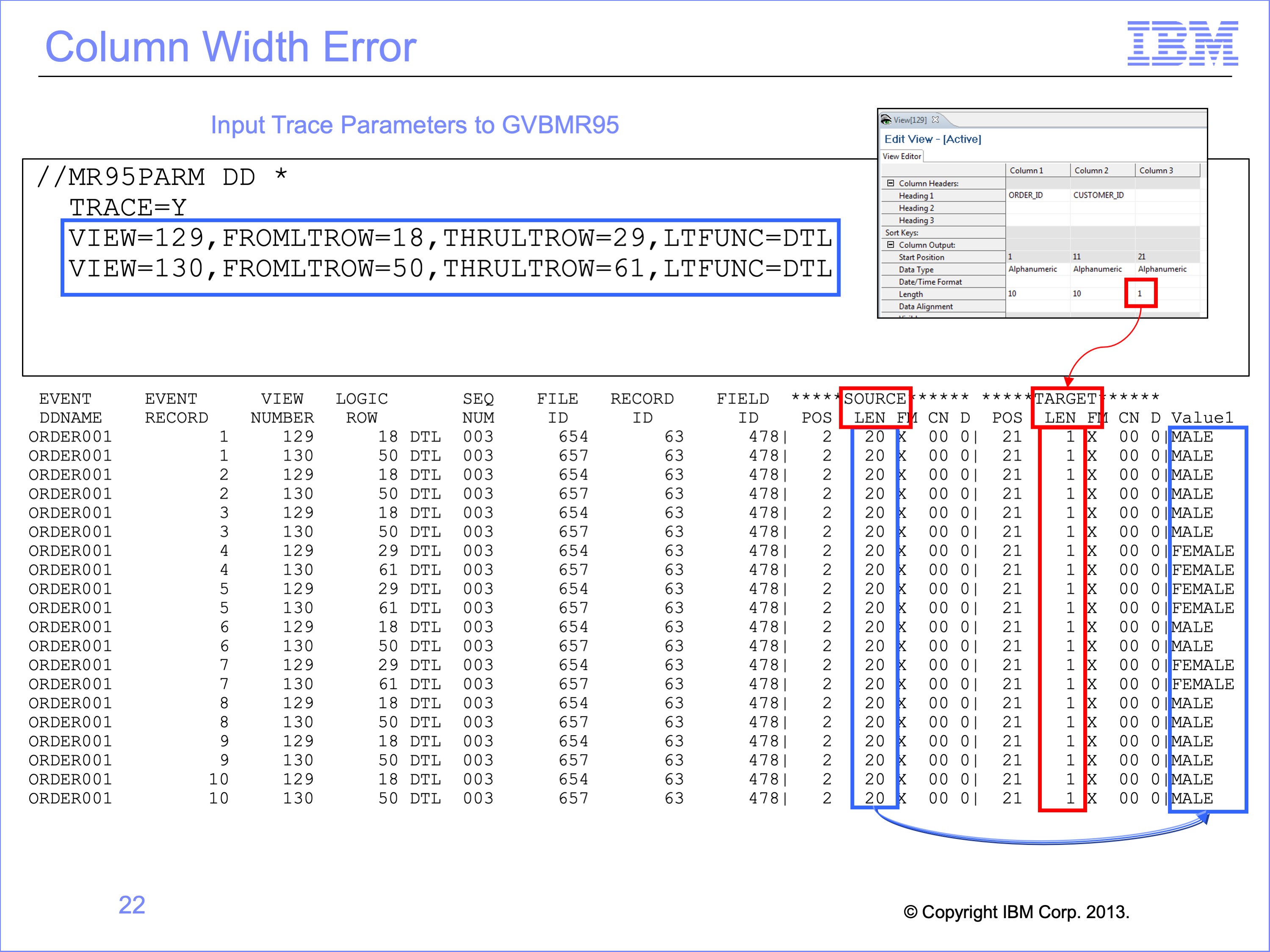
When we inspected the output, we noted it only contained the letters “M” and “F” on the end of the file, not the full reference file title values of “MALE” and “FEMALE”. If we set our trace parameters to trace only the DTL functions associated with the last column shown in this example, the trace output shows the Value 1 for the DTL function code is a 20 byte source values of “MALE” and “FEMALE” from the full reference file field. However, the Target length is only 1 byte long. The field has been truncated because the view definition was coded incorrectly. Adjusting the view column width and re-running it should correct the error.
Slide 23
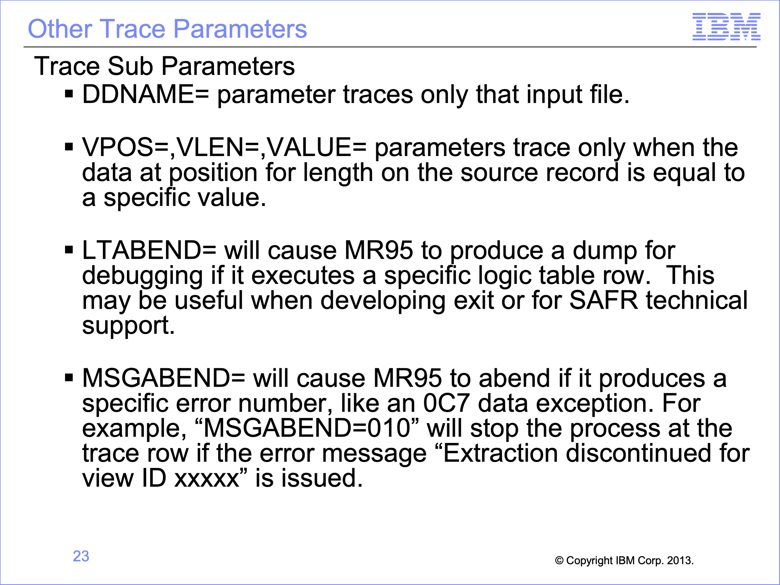
The following are descriptions of other trace parameters we have not examined in detail in this module.
- The DDNAME parameter will trace only the specified input file. While the TRACEINPUT shows input record for a DD Name, this parameter shows only executed logic table rows against that file.
- The VPOS, VLEN, and VALUE parameters trace only when the data at position for length on the source record is equal to a specific value. These parameters can consume a great deal of CPU resources against very large files. Use them with care.
- LTABEND will cause GVBMR95 to produce a dump for debugging if it executes a specific logic table row. This may be useful when debugging user exits which we’ll discuss in a later module.
- And MSGABEND will cause MR95 to abend if it produces a specific error number, such as an 0C7 data exception.
Slide 24
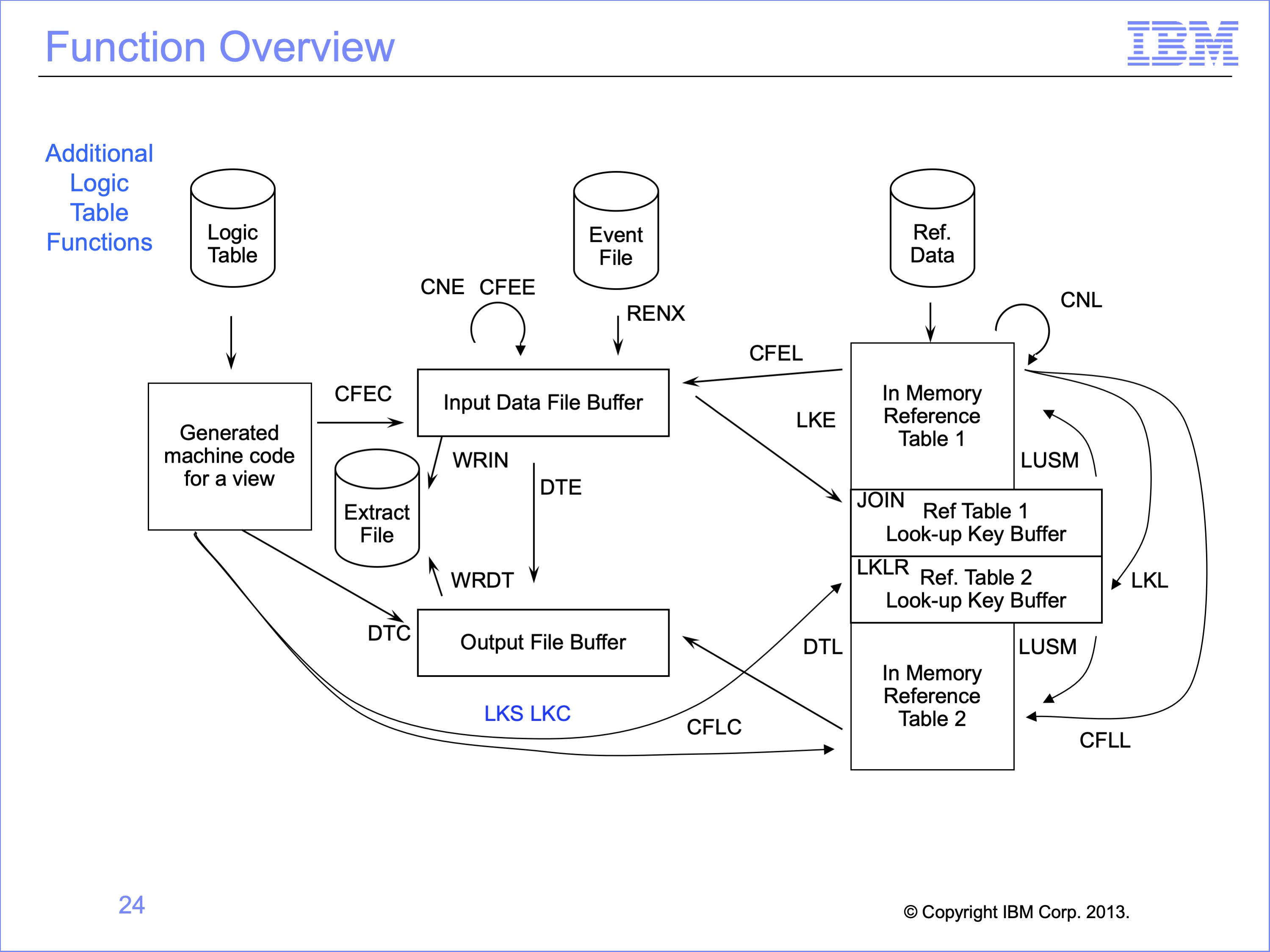
This module has introduced the following Logic Table Function Codes:
- LKC, builds a look up key using a constant
- LKS, builds a look up key using a symbolic
Slide 25
This module described lookups with constants and symbolics . Now that you have completed this module, you should be able to:
- Read a Logic Table and Trace with constants and symbolics in lookup key fields
- Explain the Function Codes used in the example
- Debug lookups with symbolics
- Use selected Logic Table Trace Parameters
Slide 26
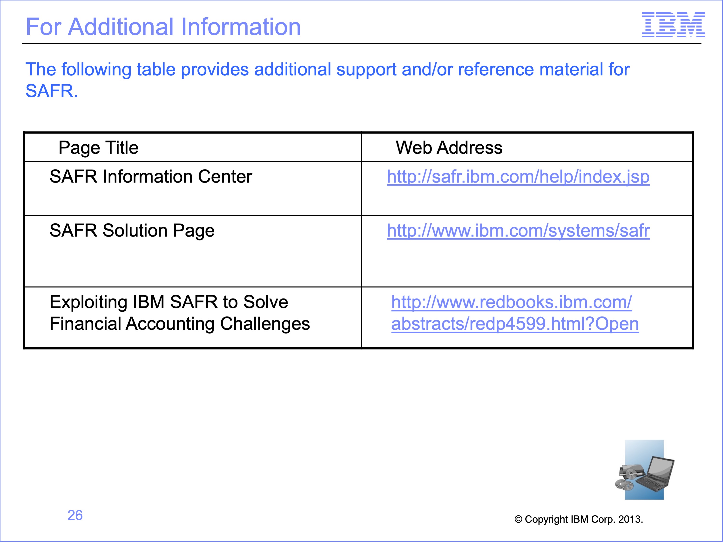
Additional information about SAFR is available at the web addresses shown here. This concludes Module 15, Lookups using Constants and Symbolics
Slide 27