The slides used in the following video are shown below:
Slide 1

Welcome to the training course on IBM Scalable Architecture for Financial Reporting, or SAFR. This is Module 13, Single Step Lookups
Slide 2
Upon completion of this module, you should be able to:
- Describe the Join Logic Table
- Describe the advantages of SAFR’s lookup techniques
- Read a Logic Table and Trace with lookups
- Explain the Function Codes used in single step lookups
- Debug a lookup not-found condition
Slide 3
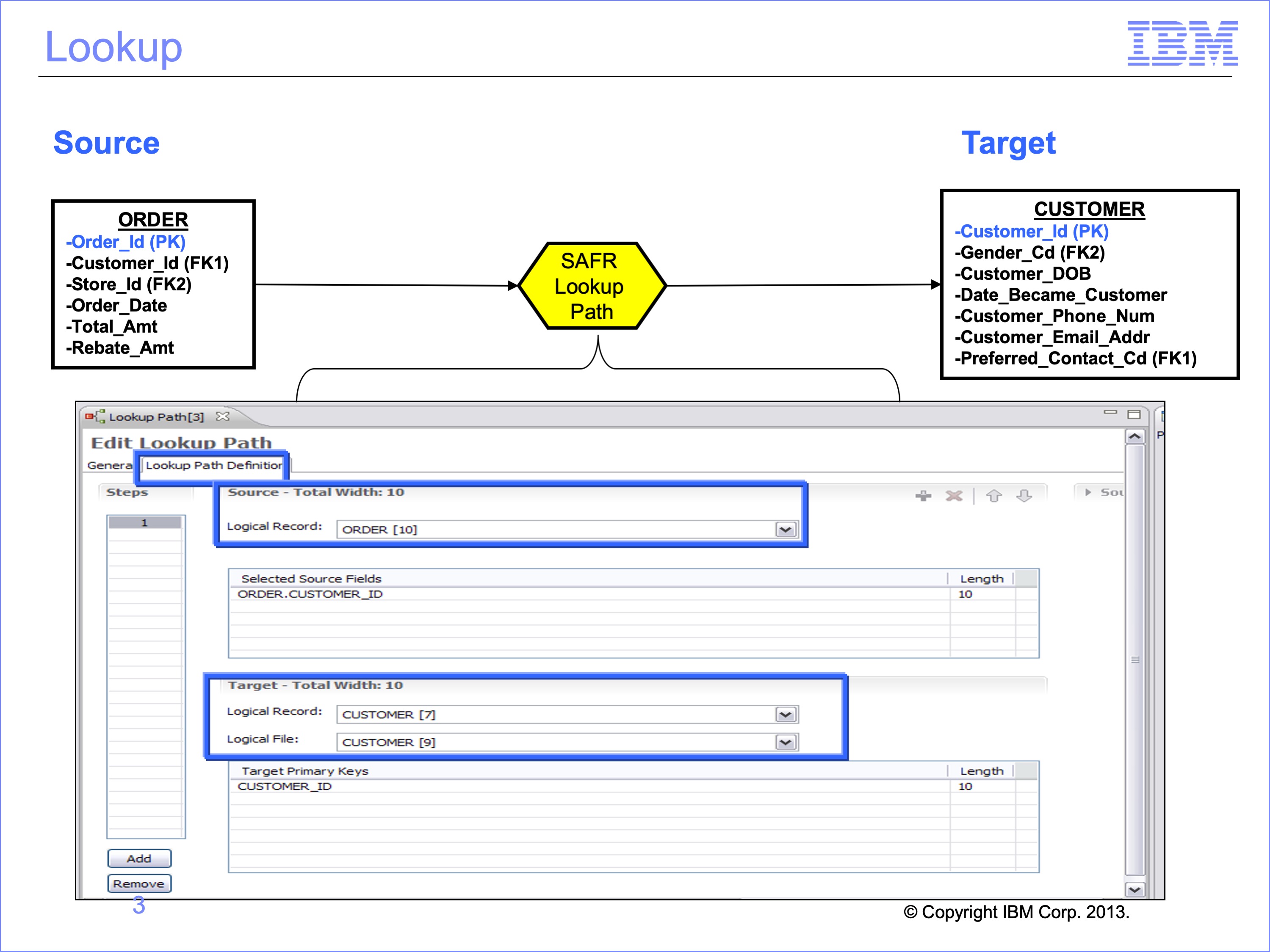
Remember from Module 4 that SAFR allows users to combine or “join” data together from different files for selection tests or inclusion in an output file. Joins or Lookups require a Lookup Path to instruct SAFR which data from the two files to match, the source and the target. The fields in the lookup path are used in the Logic Table to build a key which is then used to search the target table for a match. All lookups begin by using fields from the Source or Event LR or constants.
Slide 4
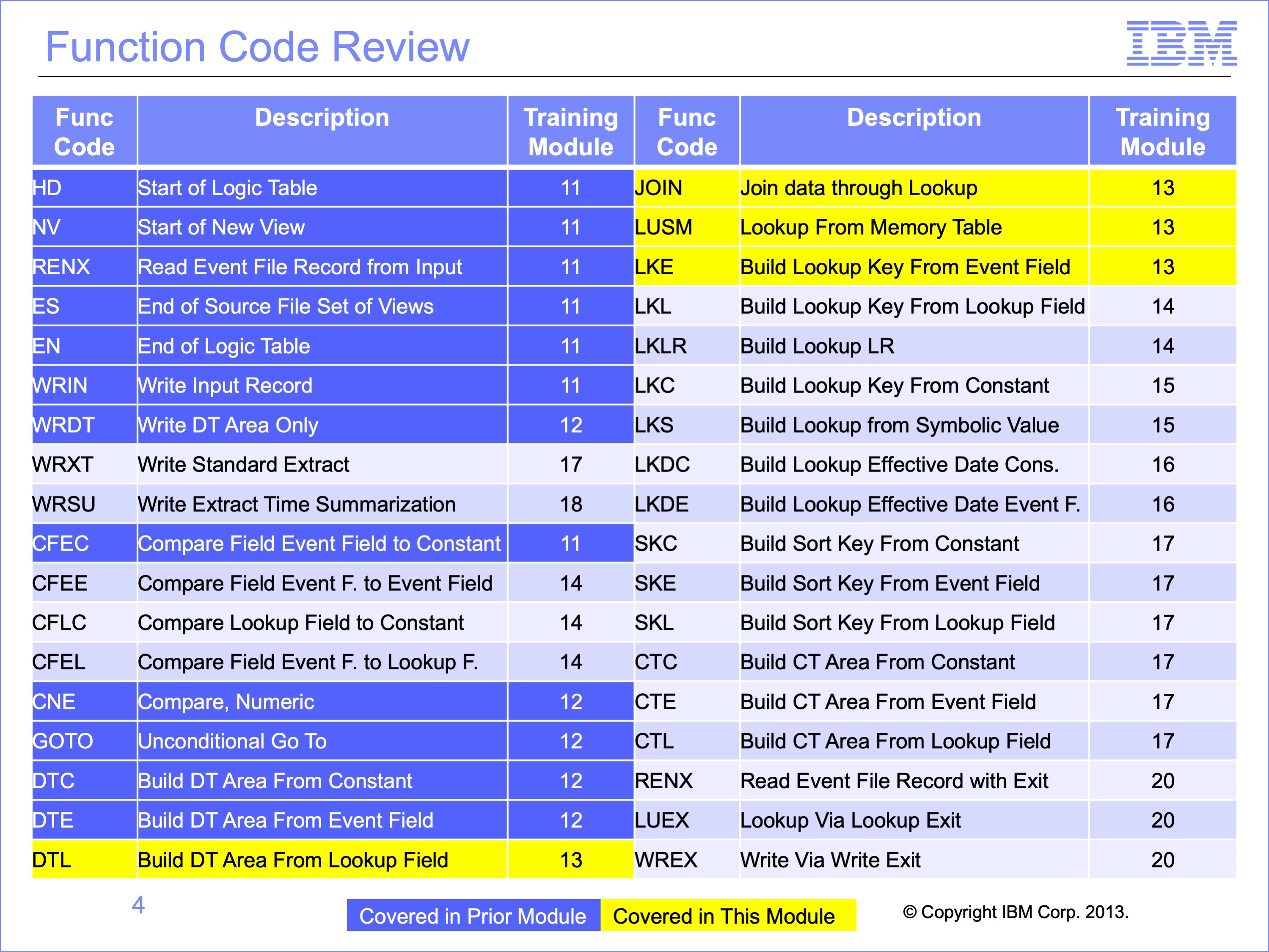
The prior modules covered the function codes highlighted in blue. Those to be covered in this module are highlighted in yellow.
Slide 5
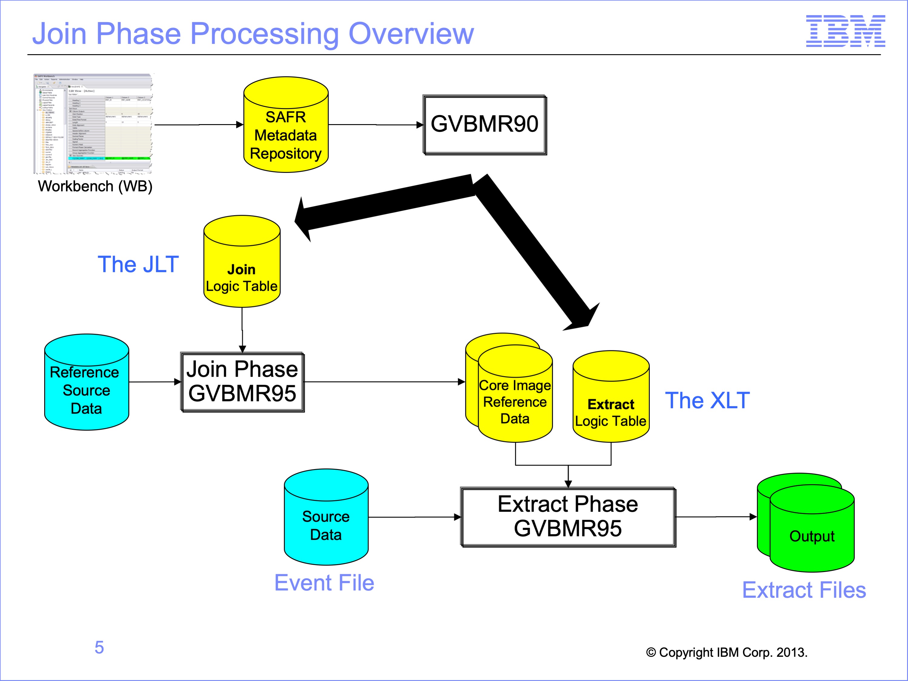
The Performance Engine flow changes when joins are performed. GVBMR90 generates two logic tables, one for use in the Extract Phase, called the XLT for Extract Phase Logic Table. This logic table contains the views selected for processing from the SAFR meta data repository. We’ve analyzed XLT Logic Tables in prior modules.
When lookups are required, GVBMR90 also generates a Join Logic Table, called a JLT. This logic table contains artificially generated views used to preprocess the reference data. These views are never stored in the SAFR Metadata repository, and are regenerated every time GVBMR90 is run.
In Join Processing, the Extract Engine is executed twice, once with the JLT and the second time with the XLT. The Join Phase GVBMR95 reads the raw Reference Data files as its source data. The outputs from the Join Phase are used in memory datasets by the Extract Phase to perform high speed joins.
Slide 6
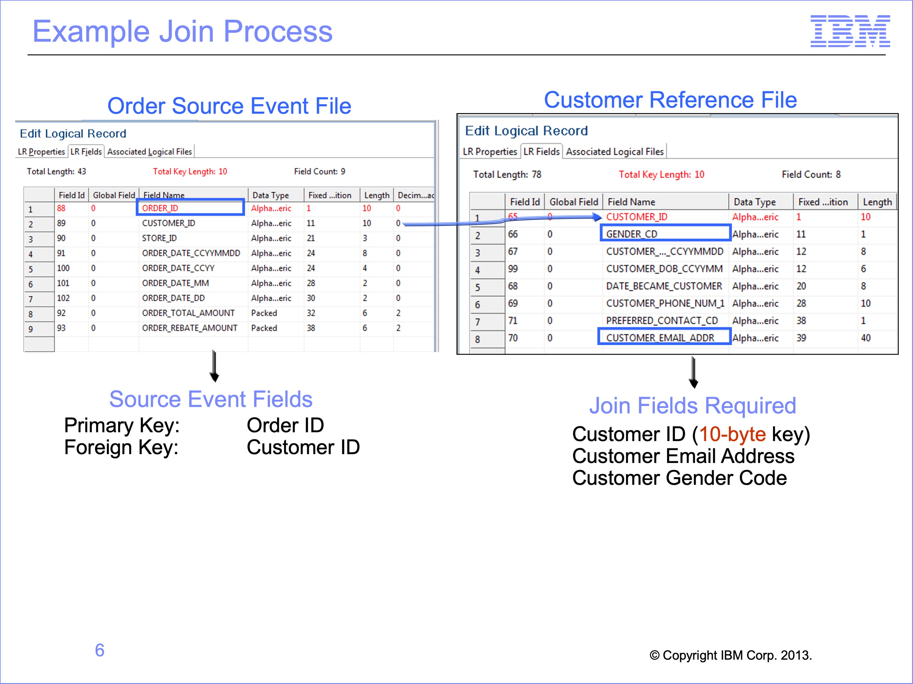
In this and following modules we’ll use a simple order example. We’ll create a file that contains the Order ID, Customer E-mail Address, and Customer Gender Code.
Available data includes
- Customer’s orders are recorded on the Order file with an Order ID as the key.
- Customer data is recorded in a separate file, keyed by Customer ID.
Each customer can make more than one Order, so the records in the Order file are more numerous than those in the customer file. SAFR is designed to scan the more detailed file as the source event file and lookup keyed data in another file. Thus we’ll define the Order file as the Source Event File, and the Customer file as a Reference File. We’ll use these files to produce our a very simple output.
Slide 7
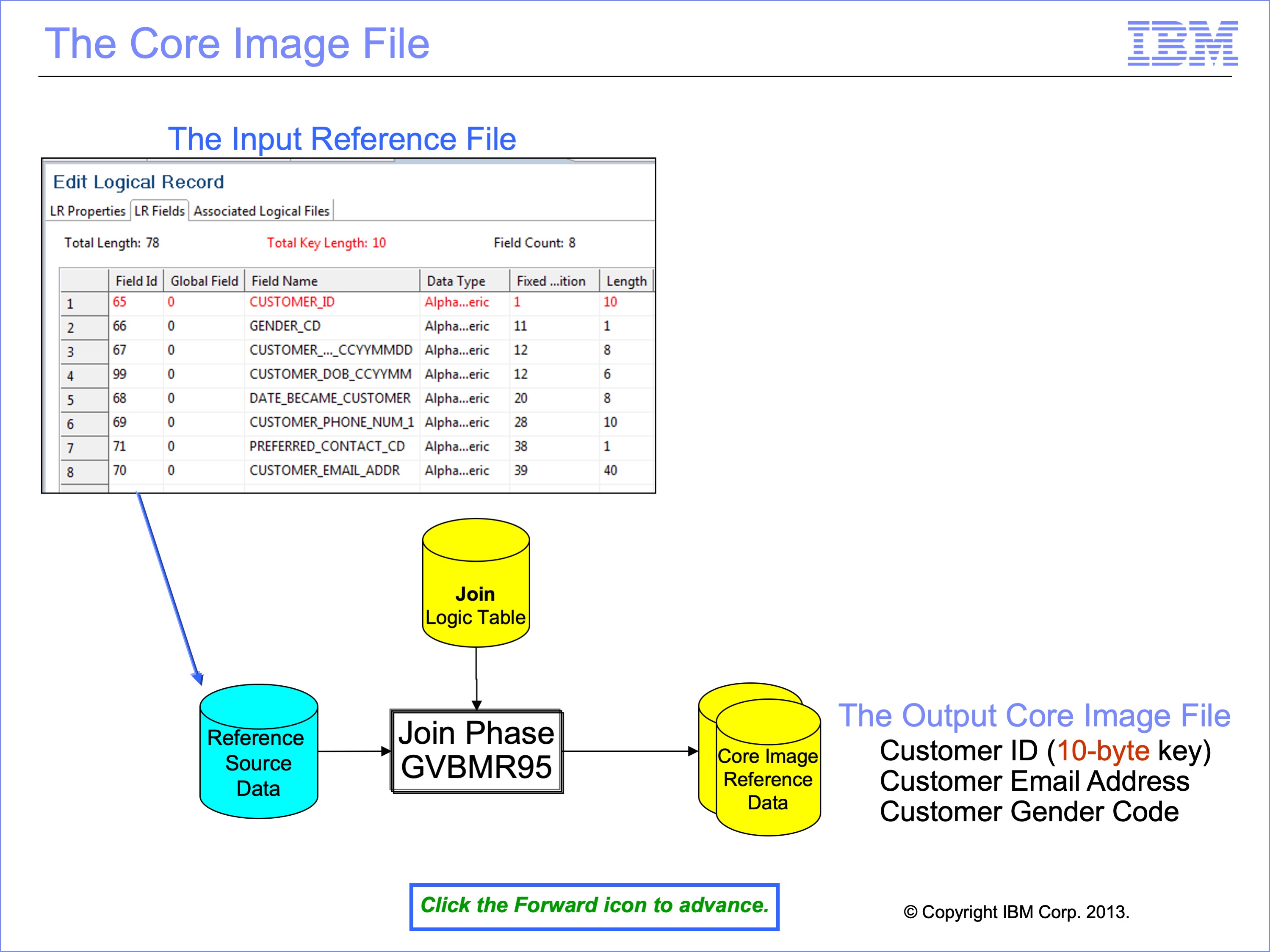
SAFR loads target join data into memory in order to increase efficiency. Memory access is thousands of time faster than disk access. However, memory is more expensive than disk. Loading the entire source reference data, including fields that are not needed, into memory can be difficult or expensive. The purpose of the JLT is to create a Core Image File, with only those fields needed for extract phase processing. In our example, only the Customer ID, which is the key to the table, and the Customer E-mail Address and Customer Gender Code fields are needed in the core image file during Extract Phase processing.
Slide 8
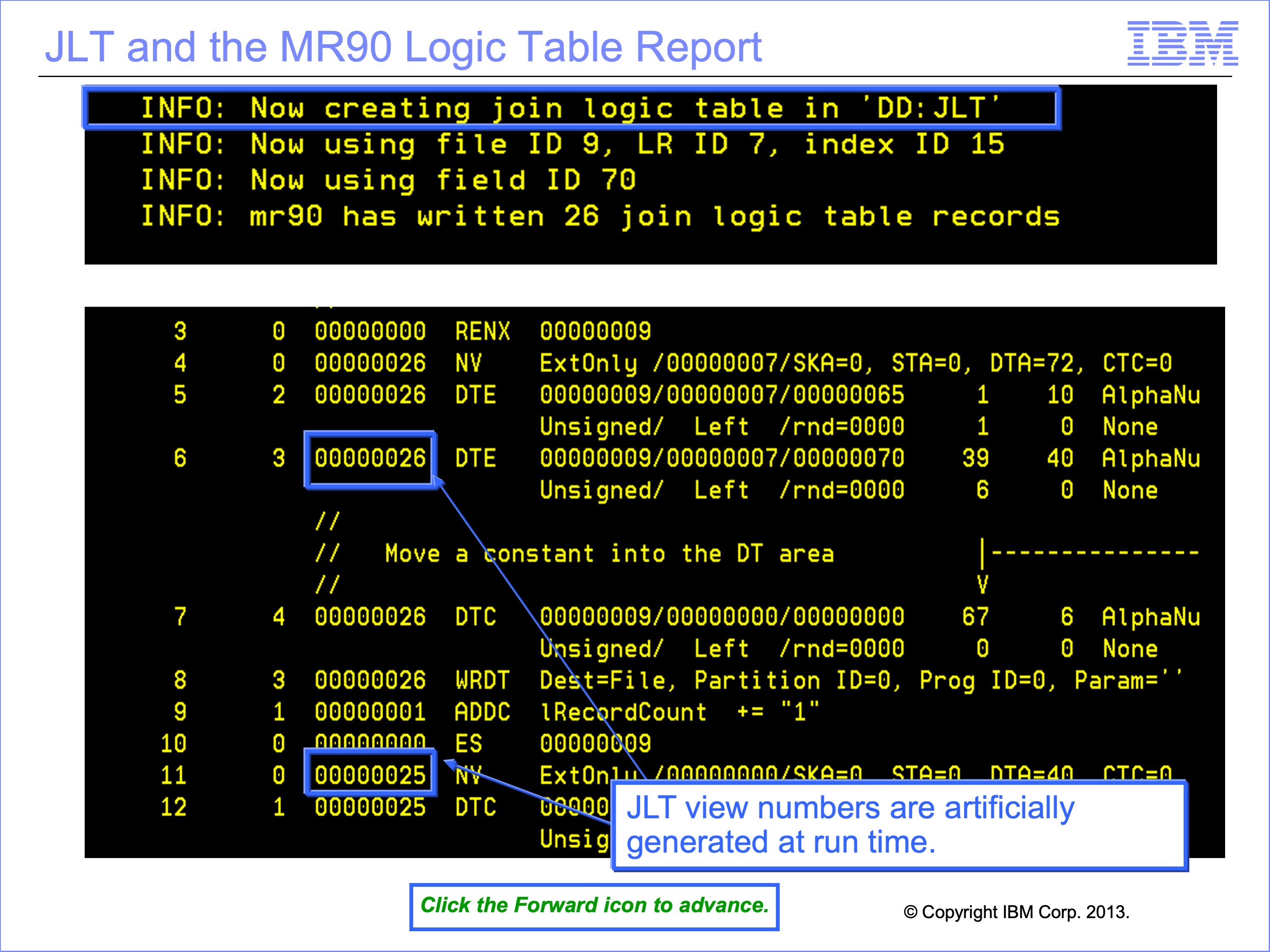
When no joins are required by any view being executed, the MR90 Control Report will show an empty Join Logic Table. When joins are required, the MR90 Control Report will contain a printed copy of the JLT.
For our example, the JLT will contain two Extract Only type views, one to extract the reference data needed in a core image file for the Extract Phase and one to create a header record. These Extract Only views are generated by GVBMR90 at run-time-only. They are never stored in the SAFR Metadata Repository. In this example, JLT views, 25 and 26 temporary views.
The core image view has three DTE Logic Table Functions, (1) for the Customer ID field, (2) for the Customer E-mail Address and (3) for the Gender Code. It will also have some DTC and other functions to properly format the core image file.
Slide 9
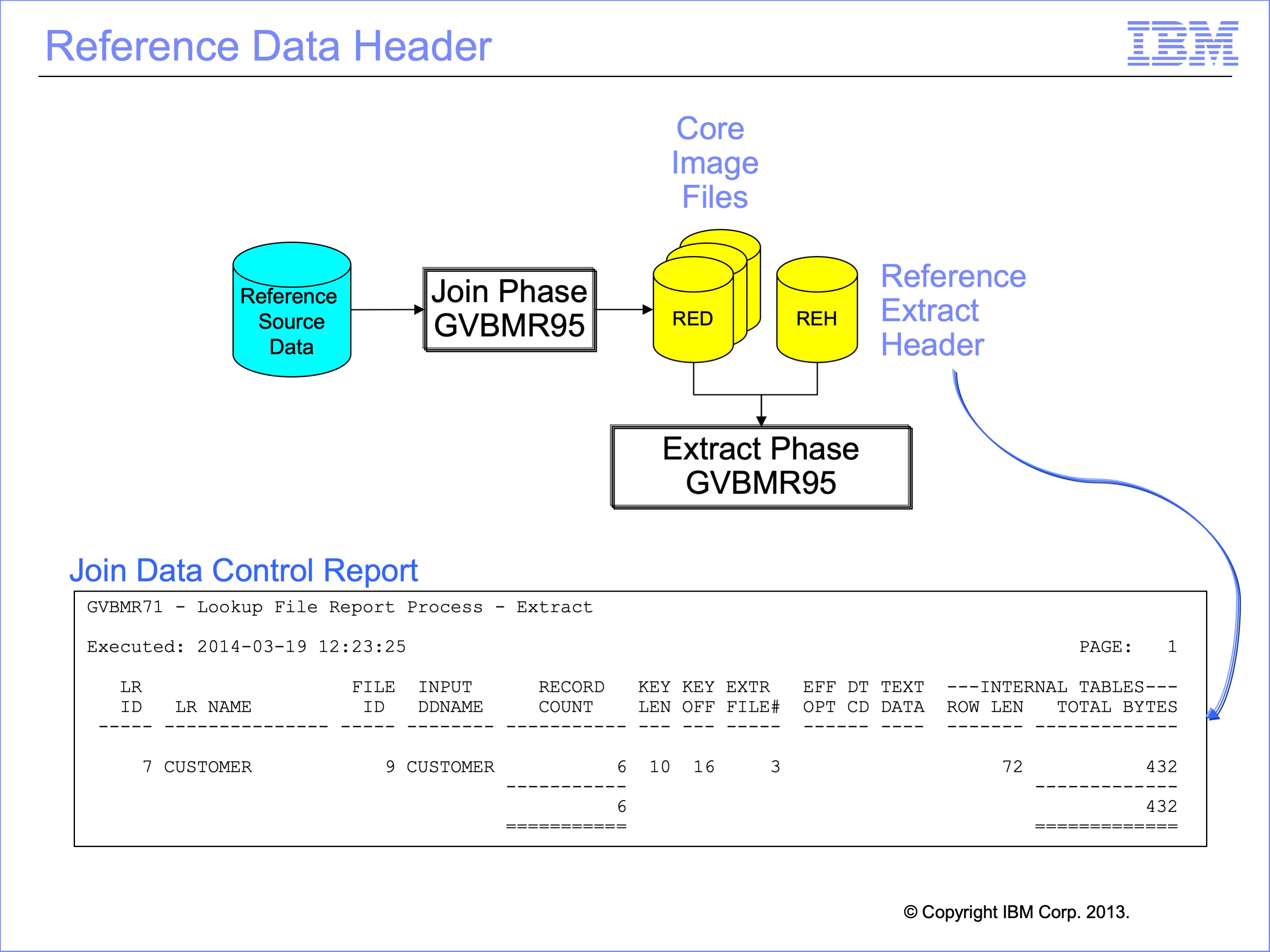
In addition the core image files, which are formally named Reference Extract Data (RED) files, the second JLT view produces the Reference Extract Header file or REH. The REH is used in the Extract Phase to allocate memory to load the Core Image Files into memory.
Each REH record contains counts of RED records and other information like the key length and offset, and total bytes required. These records are optionally printed after the Join Phase by the GVBMR71.
These control records are produced by an additional view for each reference file in addition to the Extract Only view in the JLT. This view contains some special Logic Table function codes that allow it to accumulate record counts. It also only writes one record no matter how many input records are in the reference file.
Slide 10
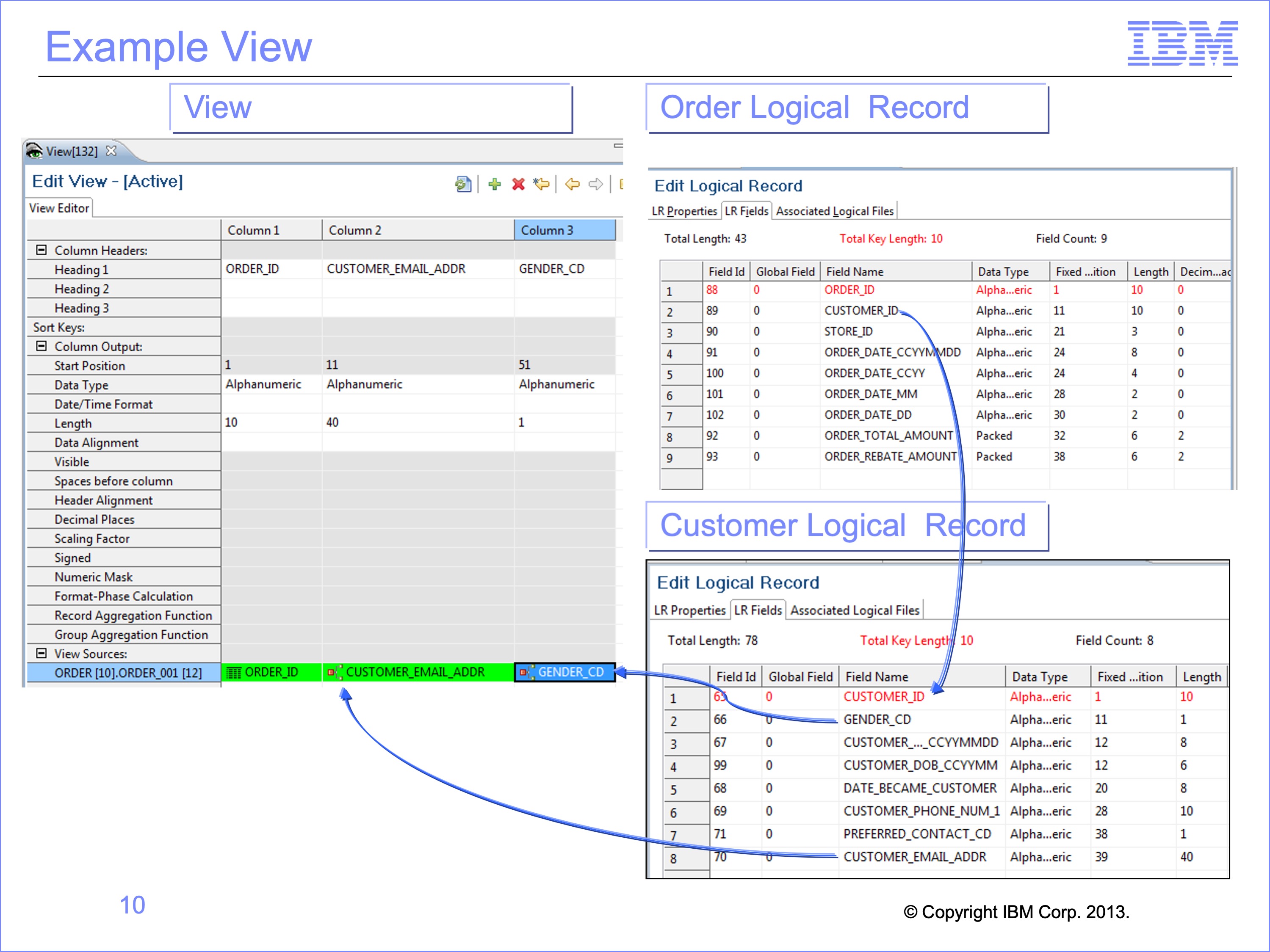
Our example look up view reads the Order logical record as the source event file. It has three columns, containing the:
- Order ID from the source event file
- Customer E-mail Address and
- Customer Gender Code, both from the Customer file
Obtaining the Customer E-mail Address and Gender requires a join to the Customer logical record. The join requires using the Customer ID on the Order logical record to search for the corresponding customer record in the Customer reference file.
As noted, the JLT will read the Customer reference file. One view will create the core image RED file which will primarily have the Customer ID and Customer Email Address field data in it. Another view will produce the REH record with a count of the number of records in the Customer core image file.
In the remainder of this module, we’ll focus exclusively on the Extract Logic Table, the XLT, for this view
Slide 11
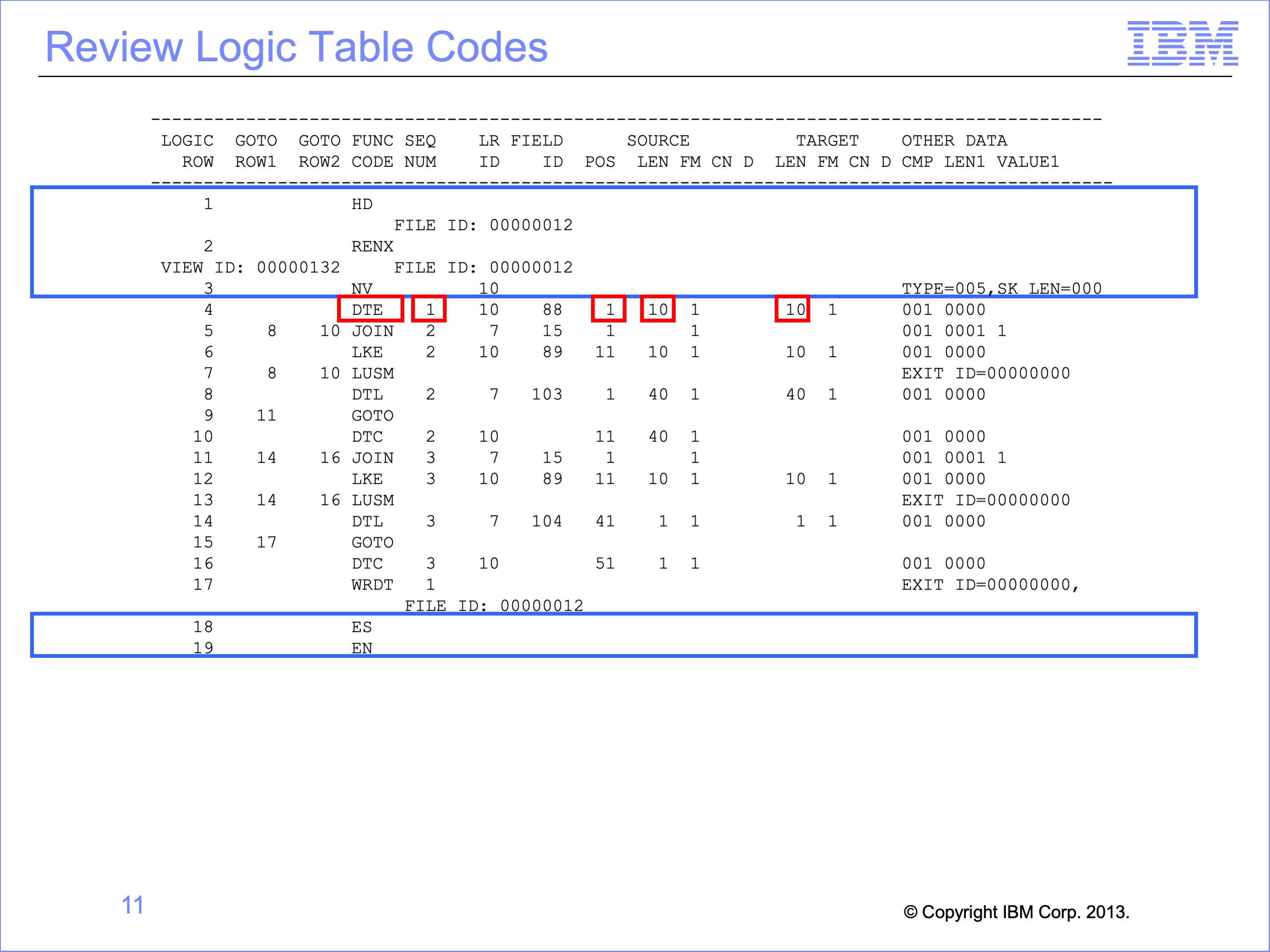
The XLT contains the standard HD Header, RENX Read Next, NV New View functions as well as the concluding ES End of Source and EN End of Logic Table functions.
Additionally, it also contains a DTE Data from Event File field function. This data is for column 1 of the view, indicated by the Sequence Number. The source data starts at position 1 for a length of 10 bytes. Under the Target section of the report, we can see that this data consumes 10 bytes in the target extract record.
Slide 12
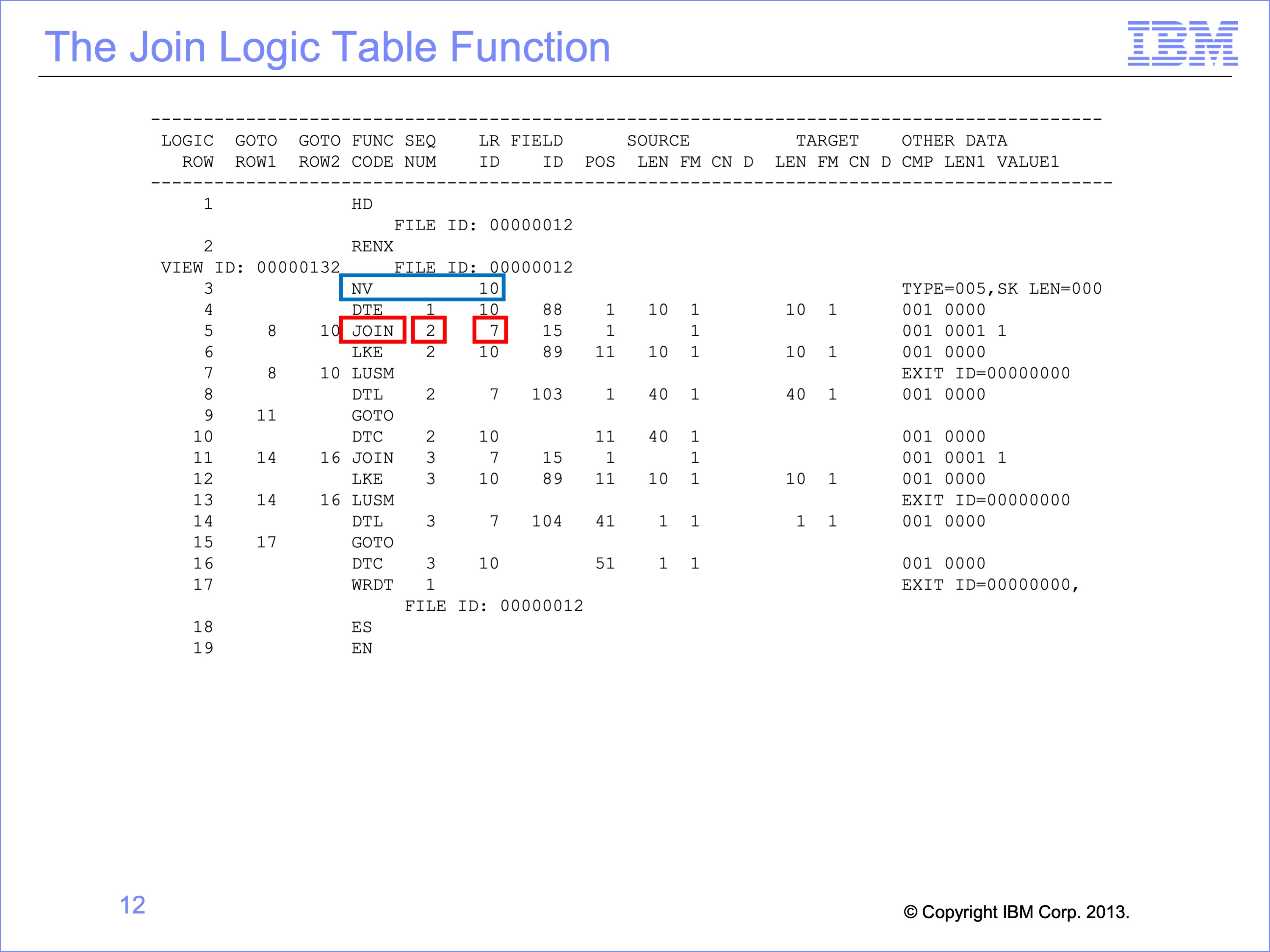
Lookups always begin with a Join function code. The Join indicates where the Lookup Path information has been inserted into the view. The steps required to perform the join are not coded in the view directly.
The Sequence number following the Join indicates which column requires this join if the logic is column specific. If the logic is general selection the sequence number will be blank. The Join also indicates the ultimate Target LR for the join.
The Join also includes Goto rows. We’ll discuss these later in this module.
In our example, The output from Column 2 is the Customer E-mail Address which requires a join to the customer file. Note that the NV indicates the source Event file LR is 10, the Order LR. The join target is LR ID number 7, the Customer reference file.
Slide 13
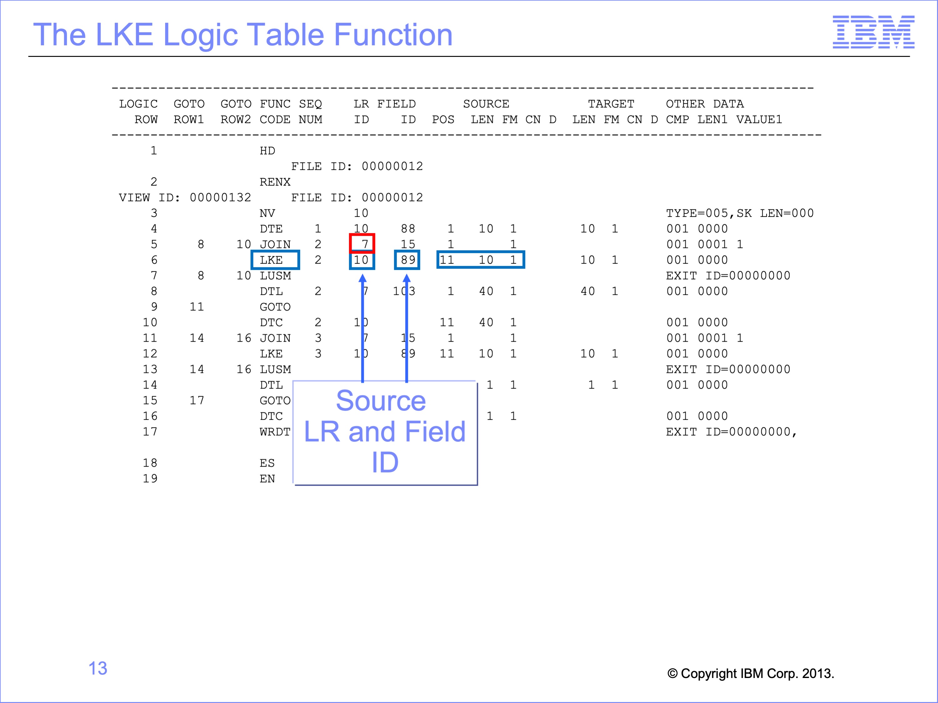
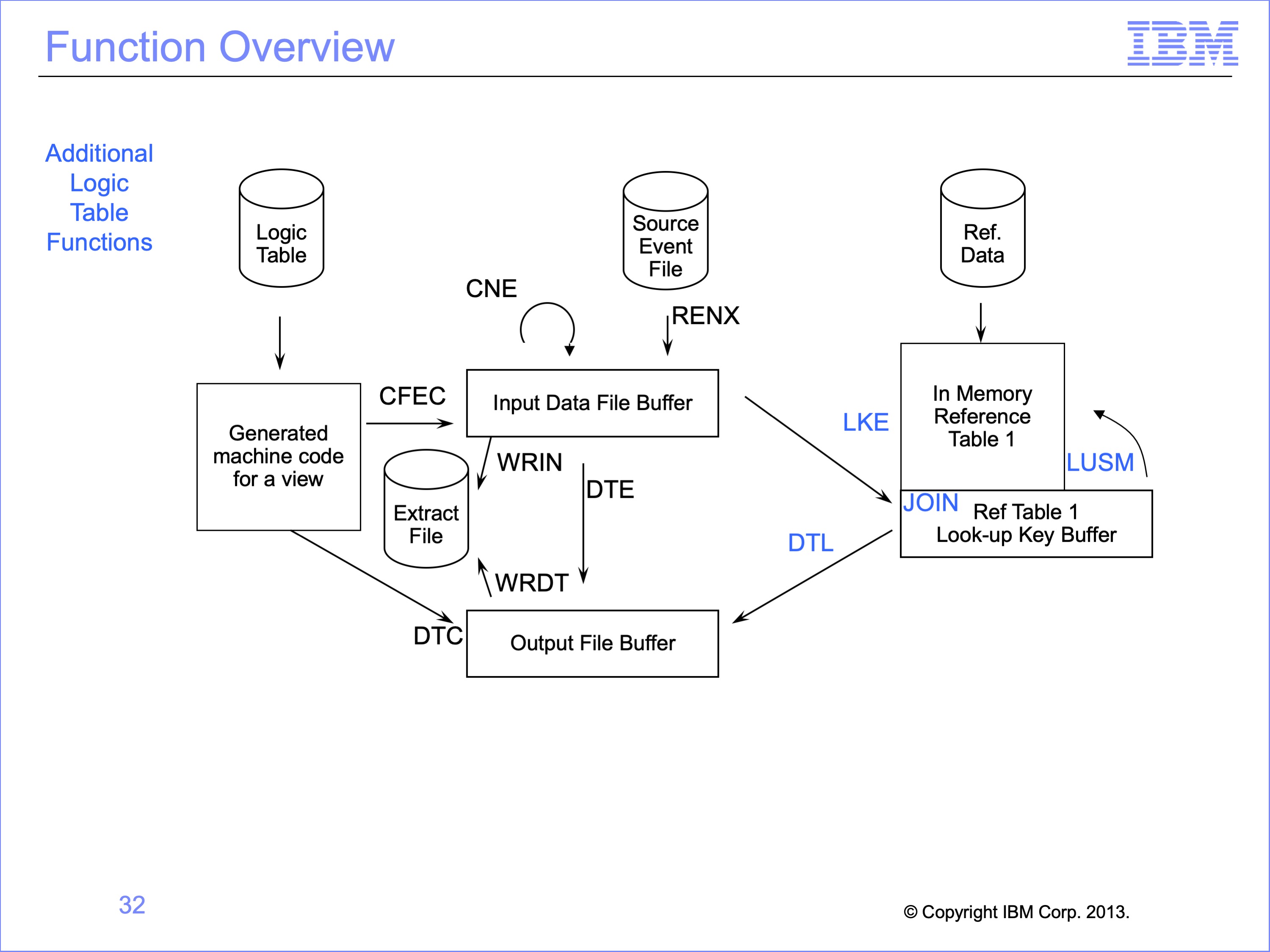
A Join is almost always followed by one or more LKE functions. An LKE function instructs the Extract Engine to build a Lookup Key from an Event File field. The LKE lists which LR the data should be taken from. The Lookup Key, as opposed to the Extract record, is temporary memory containing a key used to search the core image file for a matching value.
Note in our example that although the Join function Customer table Target LR ID is 7, the data for the key build should be taken from LR ID 10, the Order file Customer ID field. This data is found on the source record at position 11 for a length of 10 bytes.
Slide 14
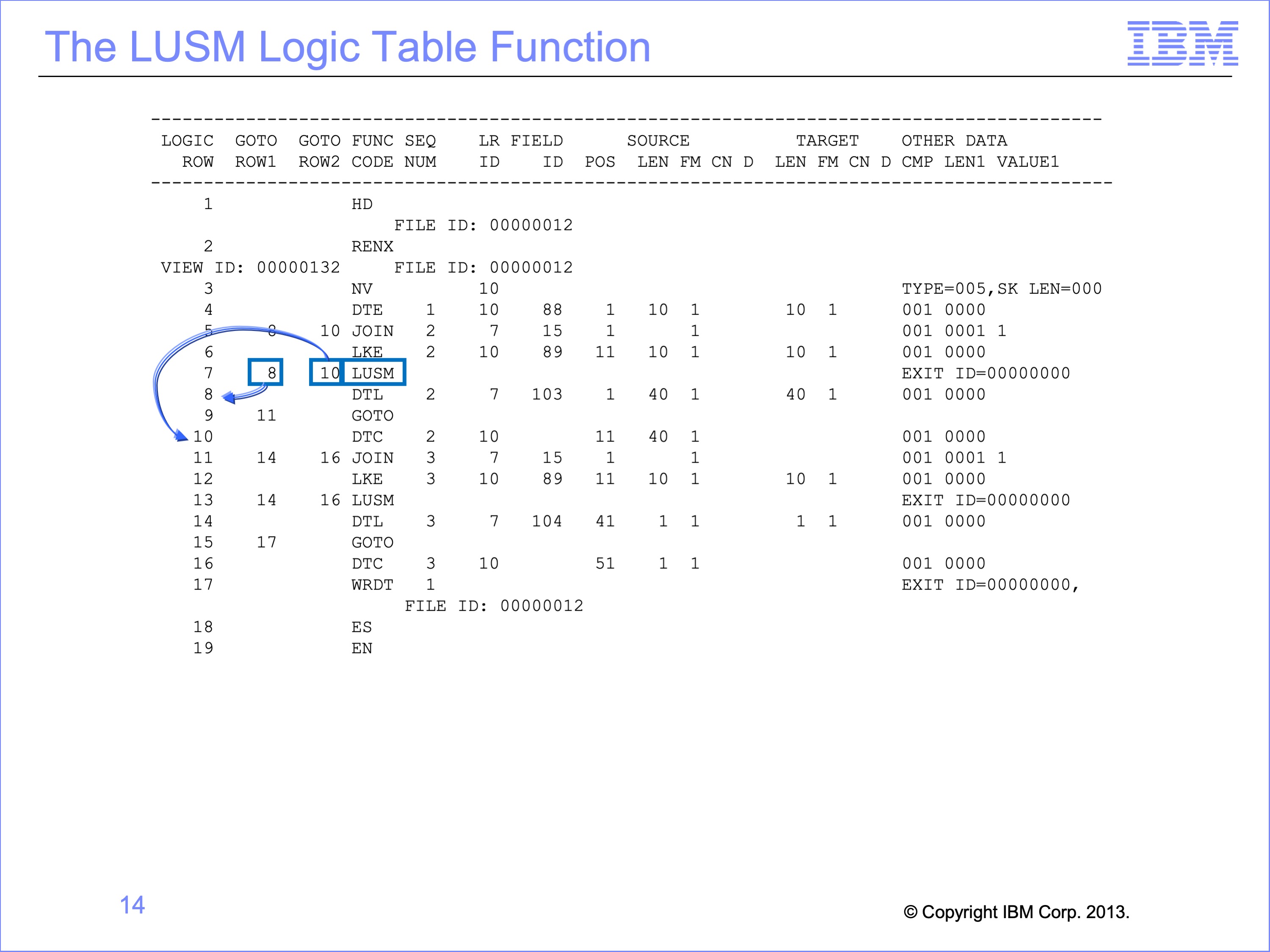
The end of a Join typically has an LUSM. The LUSM function does the binary search with the key against the Join’s target table in the RED Core Image file to find a matching record. The function code stands for Lookup to Structure in Memory.
The GOTO rows for the LUSM function are Found and Not Found conditions. Execution branches to GOTO Row1 if a reference table matching record is found for the LKx function built key. Execution branches to GOTO Row2 if no matching record is found in the reference structure.
In this example, if a matching Customer record is found for the supplied Customer ID, execution will continue at LT Row 8. If no customer is found, row 10 will be executed.
Slide 15
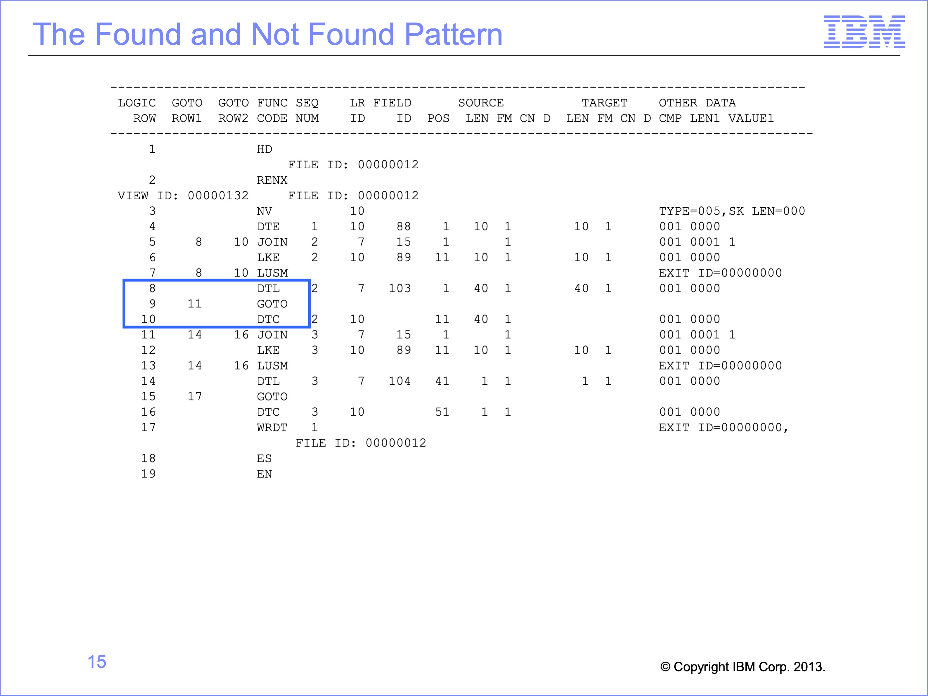
LUSM functions are typically followed by a set of functions similar in structure to the CFxx functions. You’ll remember that if the comparison proves true, often a move Data from the Event field DTE or similar function follows, then a GOTO function to skip over the ELSE condition. The else condition is often a DTC, move Data from a Constant default value.
In this lookup example, if the LUSM finds a corresponding Customer ID in the Customer table the LUSM is followed by a DTL, move Data from a Looked-up field value. If no matching Customer ID is found, a constant of spaces will be placed in the extract file by the DTC function.
Slide 16
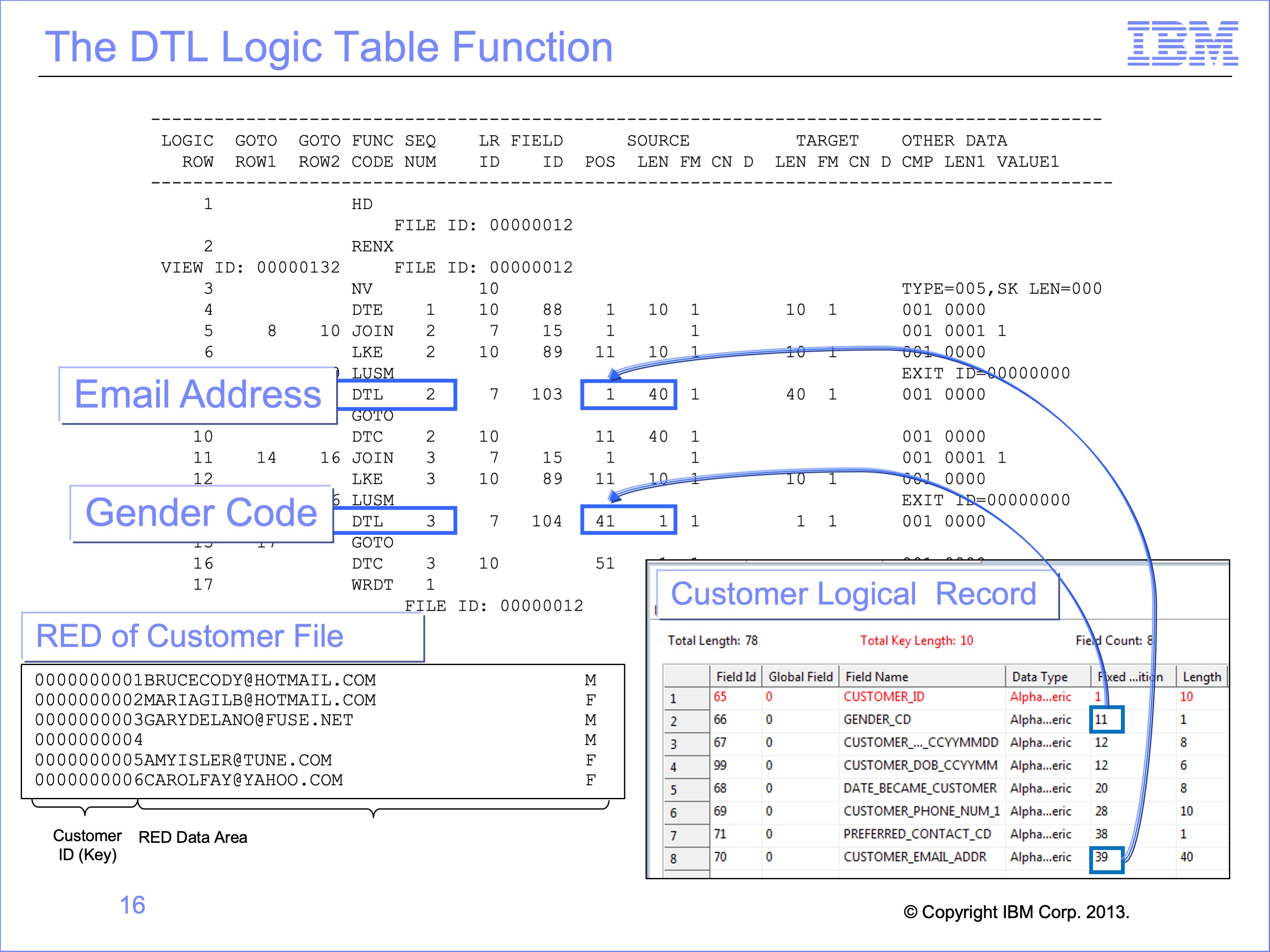
The field Source start positions on DTE functions reflect where the data resides in the event file. This is not true for the DTL functions, because the data is pulled from the RED. The data positions in the RED are not the same as the Reference Data Logical Record. The JLT process moves fields from the LR positions to the RED position, and these positions are determined by the order in which the views use the data.
In our example, the DTL function moves the 40 byte Customer Email Address on the Customer LR to the extract record from a starting position of 1 whereas on the Customer Record, it begins in Position 39.
If the LR definition of the reference file is incorrect, the RED Key and all the data may be wrong. At times it is necessary to inspect the RED file to see if the data exists.
Slide 17
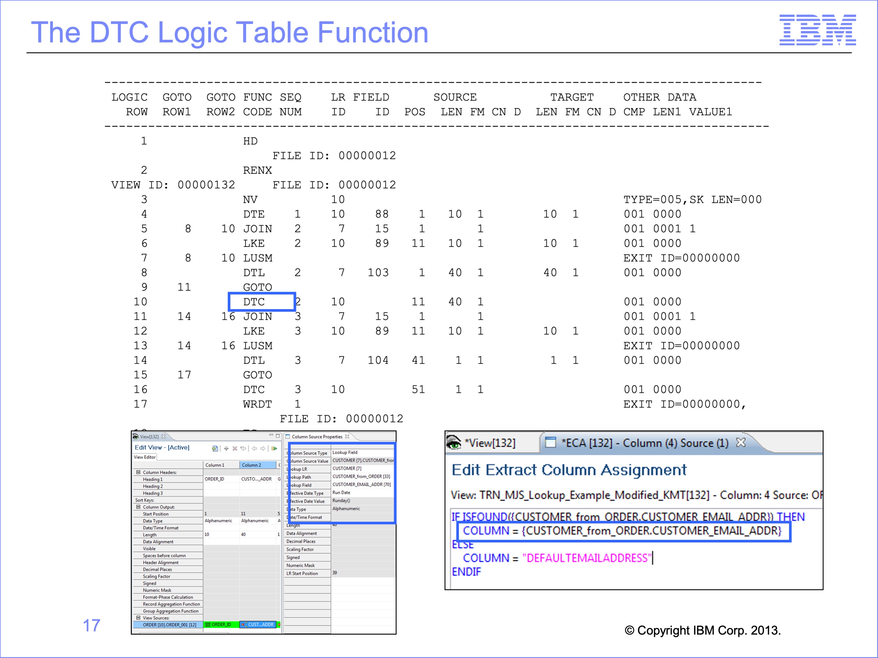
Looked-up fields can be placed in columns in two ways. They may be assigned directly, as shown in this view example and on this logic table. Or they may be coded in Logic Text.
If they are placed directed on the view editor and not in logic text, then SAFR automatically generates a default DTC in case of a not found condition. The default value depends upon the format of the target column: Alphanumeric columns receive a default value of spaces, and numeric columns a default value of zeroes.
If the field is coded in Logic Text, the user can define a default ELSE condition, which would be assigned to the DTC value.
In our example, the default value is spaces supplied by the DTC function if the lookup fails and no customer Email Address is found.
Slide 18
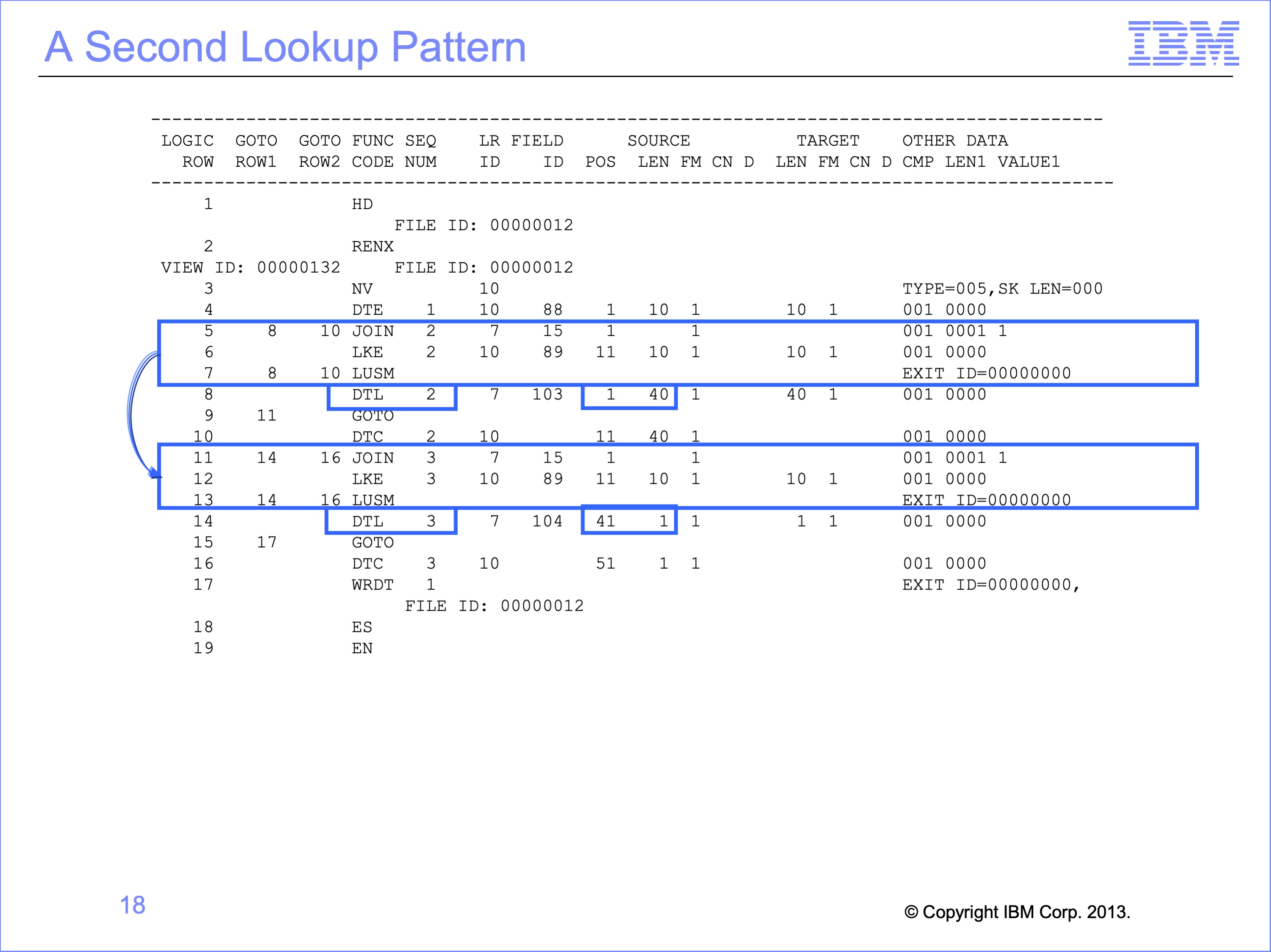
Lookup paths are often reused within views, which means lookup logic is often repeated.
Our view requires two look ups, one for the Customer Email Address for column 2, and a second for the Customer Gender Code in column 3. After the first lookup, the logic table then contains very similar logic for the second look up. Except for changes in logic table and GOTO rows and Sequence (column) numbers the second set of Join, LKE and LUSM functions are identical to the first set.
The DTL, GOTO and DTC functions are also very similar between the two lookups, with same row and sequence number differences, yet their source field and target positions and lengths also differ.
Slide 19

The first goal of SAFR is efficiency. Developers recognized that repeating LKx key build and the binary search LUSM function over and over again for the same key was inefficient, particularly when this lookup had just been performed and would have the same results. SAFR has just found the Customer record with the Customer E-mail Address, and can use this same record to find the Customer Gender. Thus SAFR has automatic Join Optimization built-in to every lookup.
This is done through the Join function GOTO Rows. Note that the GOTO Row 1 and Row 2 numbers on the Join Function are the same as the LUSM, the Found and Not Found rows. Before the Join executes, it very efficiently test if this join has been performed for this record. If it has, the JOIN immediately branches to either the Found or Not Found row based upon the last lookup. This avoids using CPU cycles to do unnecessary work.
This optimization is not limited to repeat joins within a view, but operates across all joins for all views being run against the same source event file. The greater the number of views and joins, the greater the efficiencies gained.
Slide 20
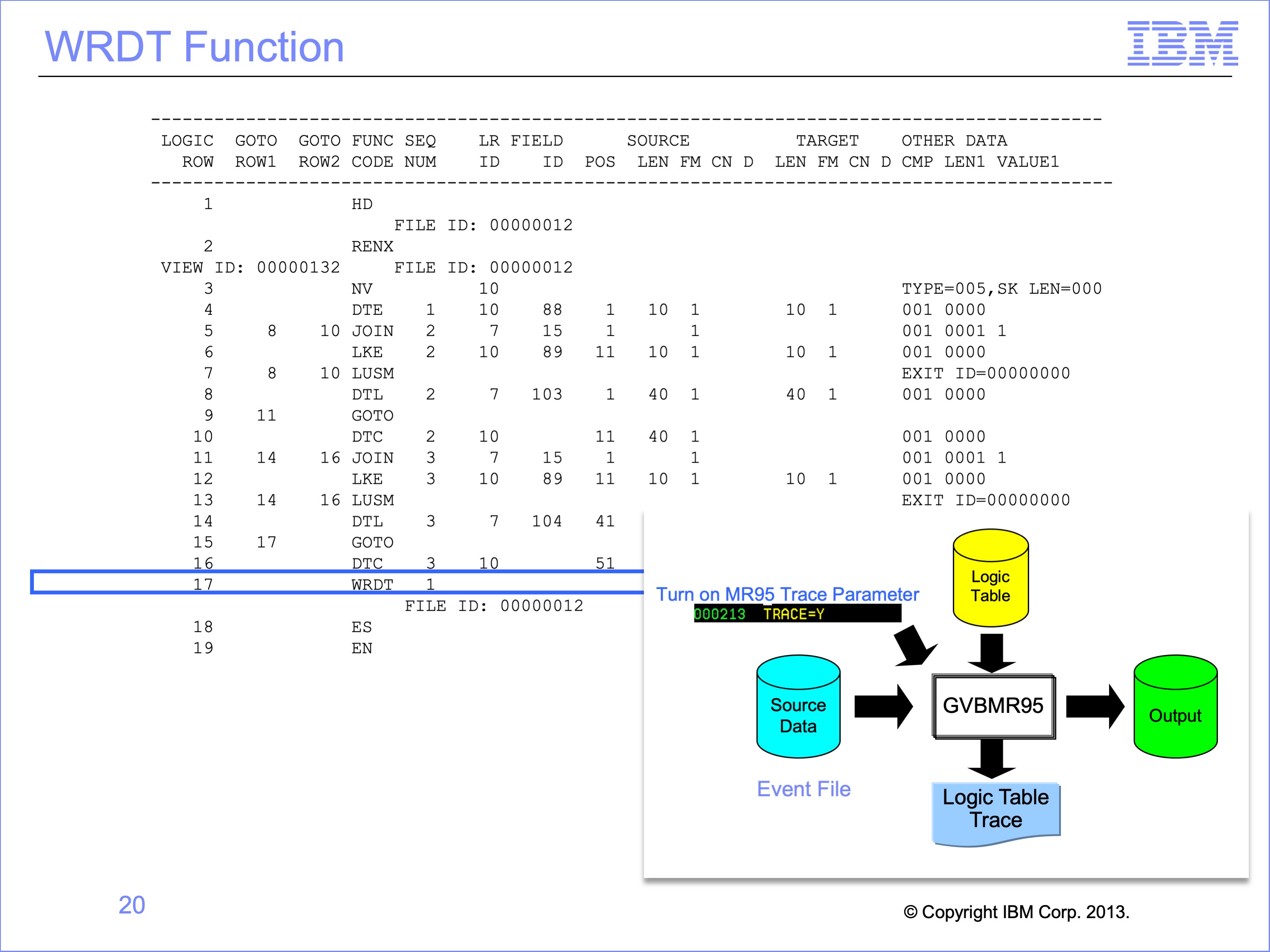
The last view specific logic table function is the WRDT, which Writes the Data section of the Extract record. The record will include the DTE data for Order ID, the DTL Customer Email Address or DTC spaces if there is not one, and the DTL Customer Gender Code or DTC spaces if that is missing.
Having examined the simple lookup logic table, let’s turn the Logic Table TRACE and examine the flow.
Slide 21
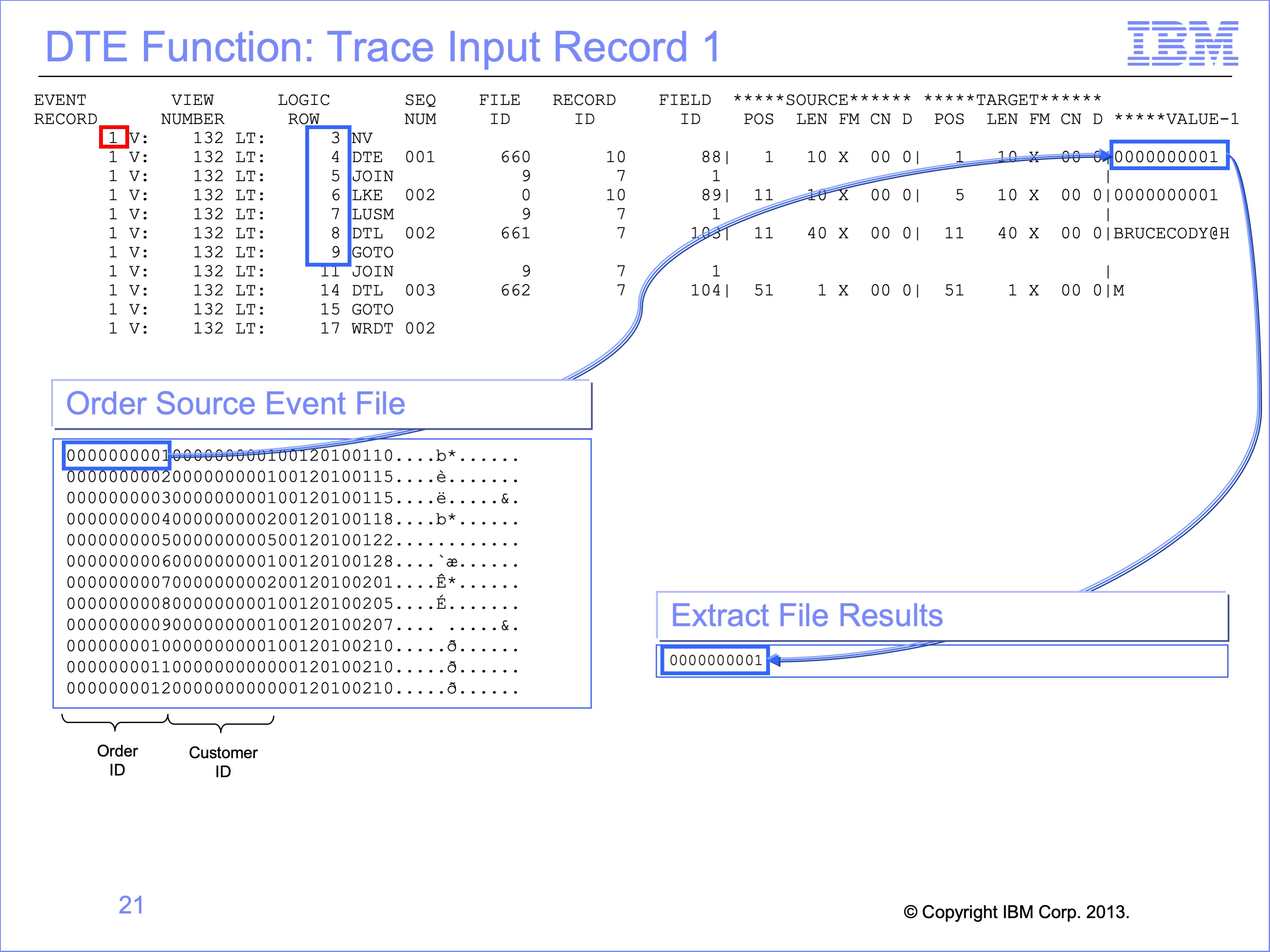
For the first record from the Order File, rows 3 through 9 are executed in order. No rows are skipped. (The HD and RENX functions of rows 1 and 2 are not shown in the trace).
The Trace shows the DTE function moving the Order ID of 0000000001 from the Order Source Event File to the Extract record.
Slide 22
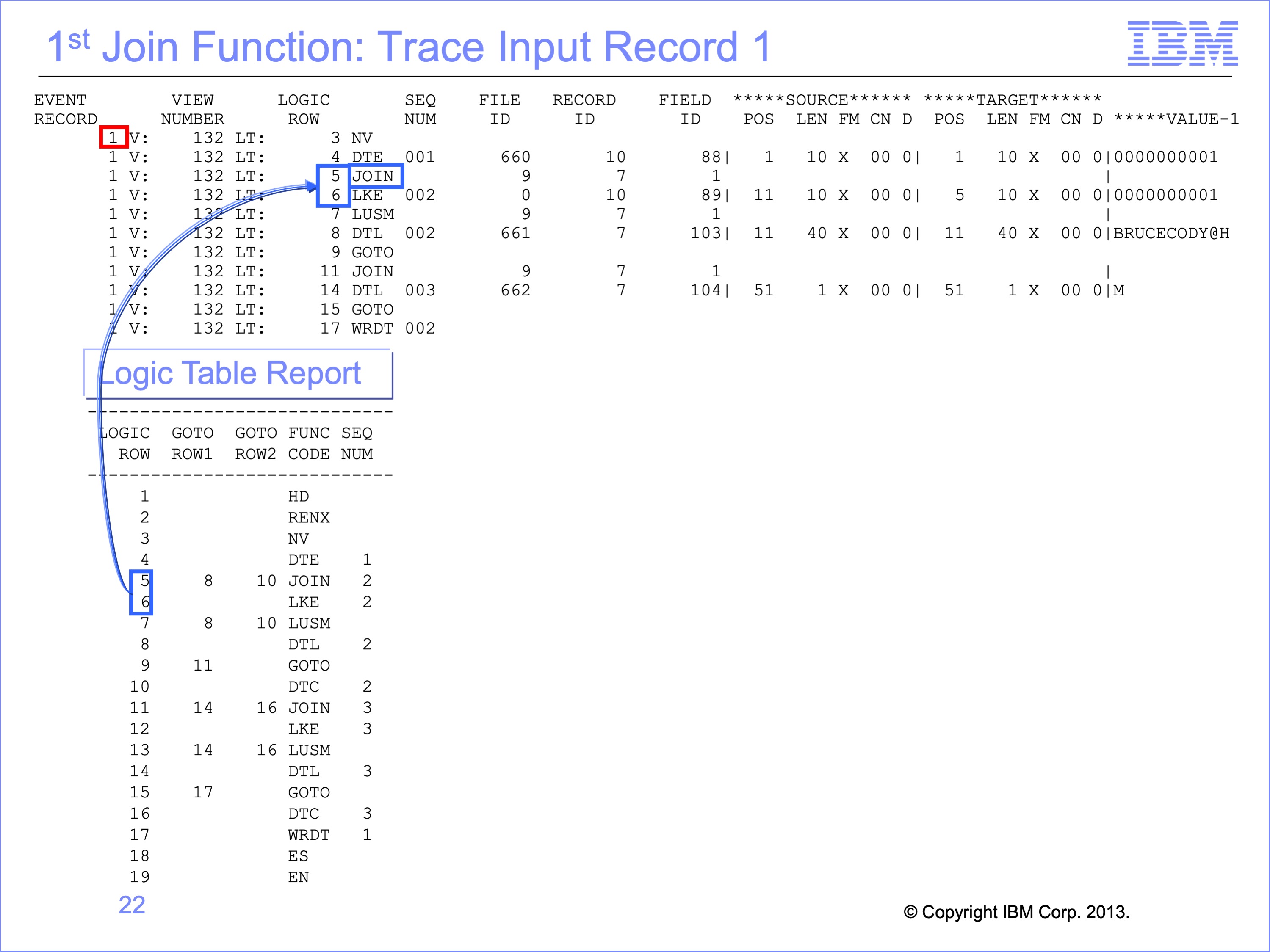
Because this is the first source event file record read, and the Join function on row 5 is the first join in the logic table, no join has been performed. The Join performs a test to see if the join has been performed, and finding that it has not, the Join falls through to the LKE function to build the key for the join. No branching from the Join is performed.
Slide 23
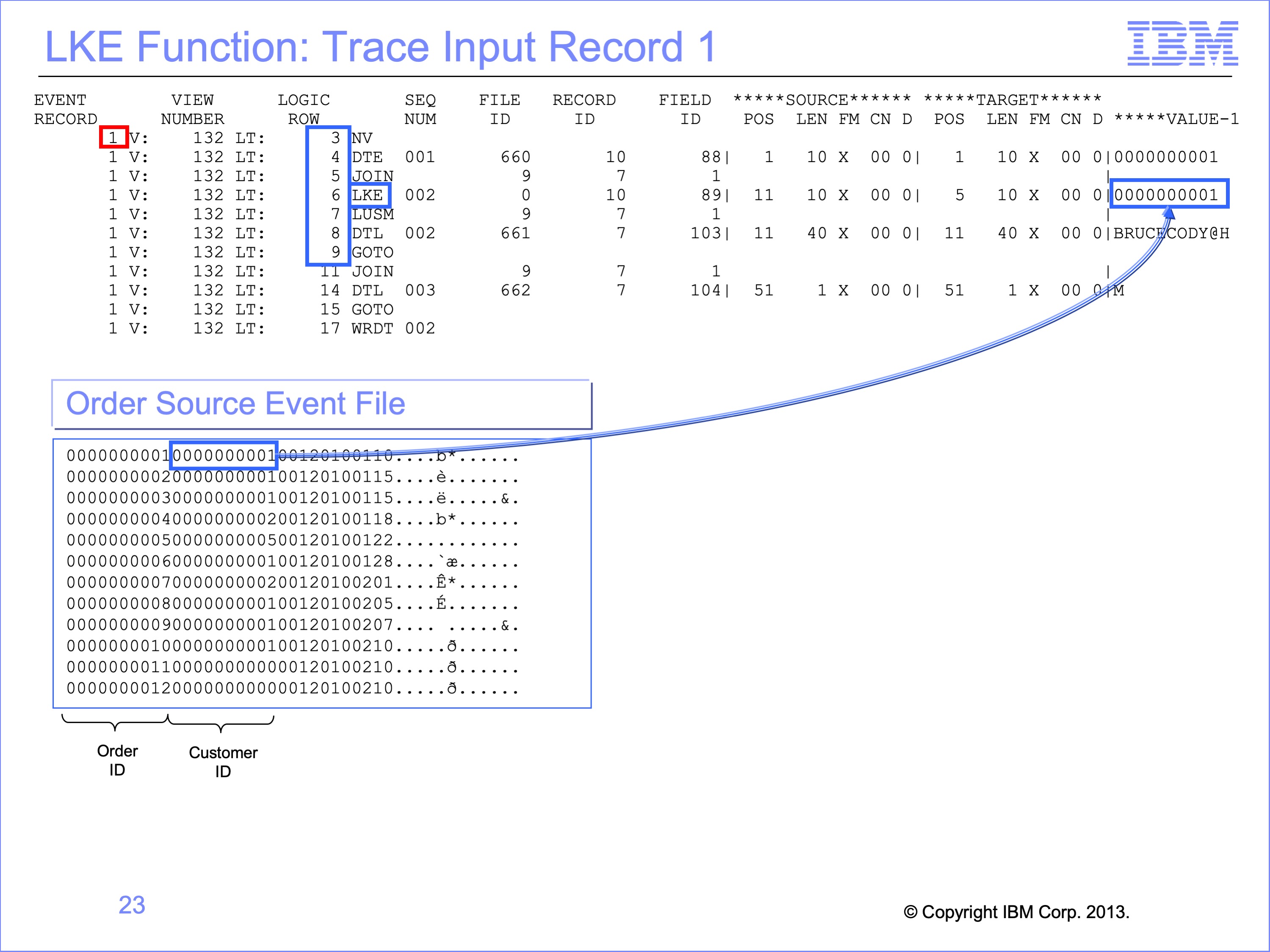
Because this is the first Join, the LKE function is used to build a key to search for a matching customer record. The trace shows the LKE value in the Customer ID field on Order file, which is moved to the lookup key buffer prior to doing the search. The search LUSM function will search for customer number 1.
Slide 24
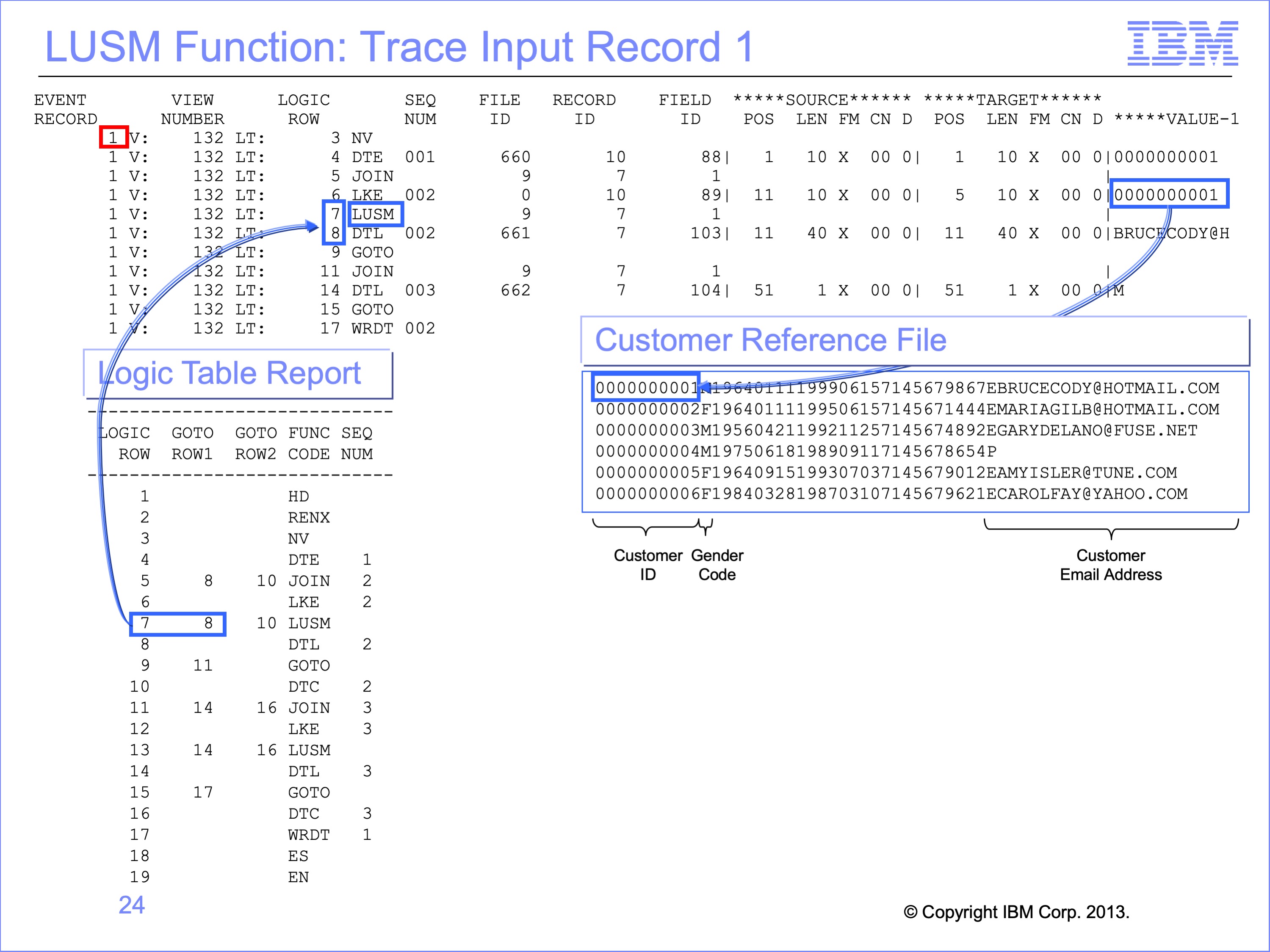
The results of the LUSM binary search can be seen by noting the next row executed. In our example row 8 is the next row in the trace; from this it is clear that the LUSM function found a corresponding customer record with customer ID 1 in the Customer Reference File. Now any Logic Table functions that reference Customer Logical Record ID 7 (called Record ID in the Trace Report) will use this record until another LUSM is performed for the Customer Logical Record.
Slide 25
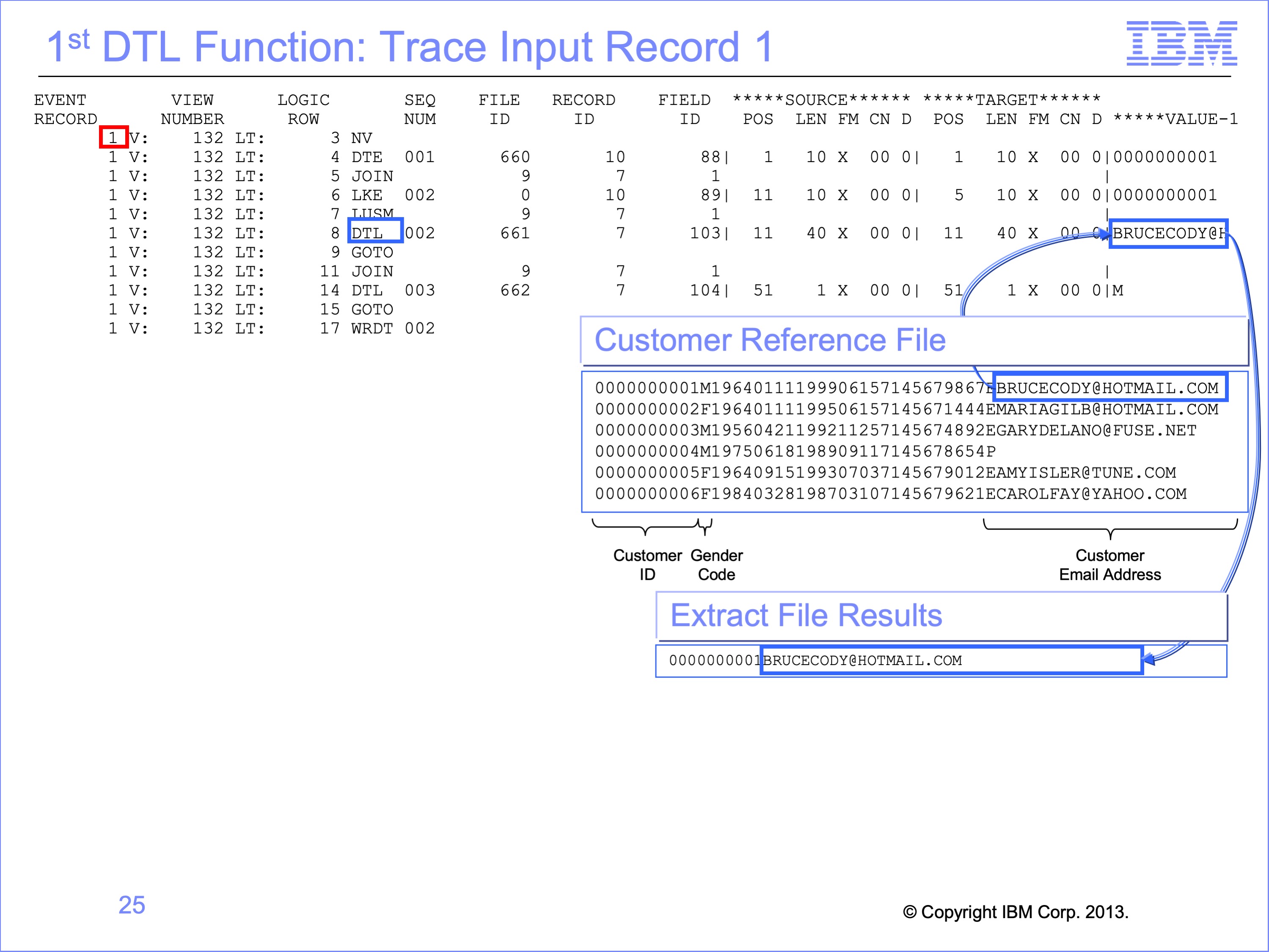
The DTL Function moves looked up data from the Customer Email Address field on the Customer Reference File to the Extract record. The trace report shows a portion of the value that is moved to the extract record.
The GOTO function on Logic Table Row 9 then skips the DTC function which would have placed spaces in the Extract record if no Customer Record had been found. Remember that the trace only shows executed logic table rows. Rows skipped are not printed in the trace.
Slide 26
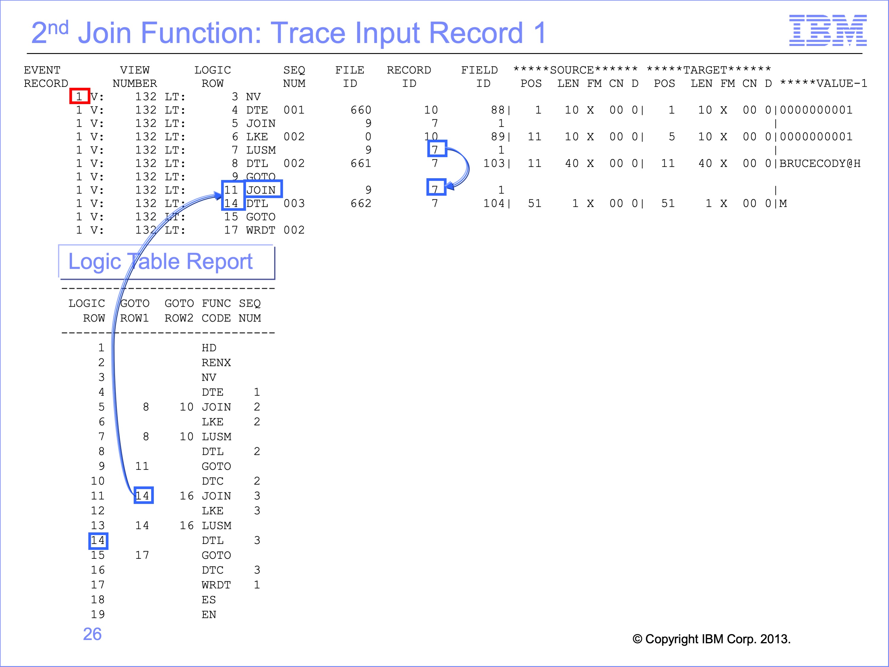
The second Join is required for the Gender code. It begins with the Join function testing to see if a join to Logical Record ID 7 has been performed previously. Since the lookup for the Customer E-mail Address was just performed and resulted in a Found Condition, the LKE, LUSM functions do not need to be performed. Rather, the GOTO Row 1 on the Join is used, just like the second LUSM had been performed and found Customer ID 1 again in the Customer record. In this particular logic table, logic table rows 12 and 13 will likely never be executed during processing.
Slide 27
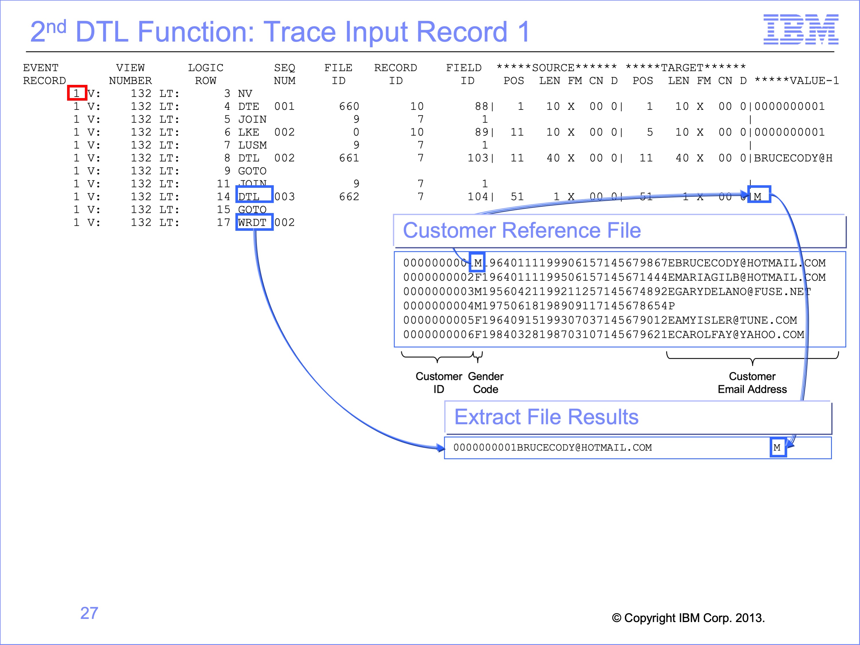
The 2nd DTL Function moves the Customer Gender code from the Customer Reference File to the Extract record. The trace report shows the “M” value that is moved to the extract record. The GOTO function on Logic Table Row 16 then skips the DTC function which would have placed spaces in the Extract record if no Customer Record had been found.
The WRDT function writes this completed Extract Record to the Extract File. Execution then resumes at the RENX function for the next Event Record.
Slide 28
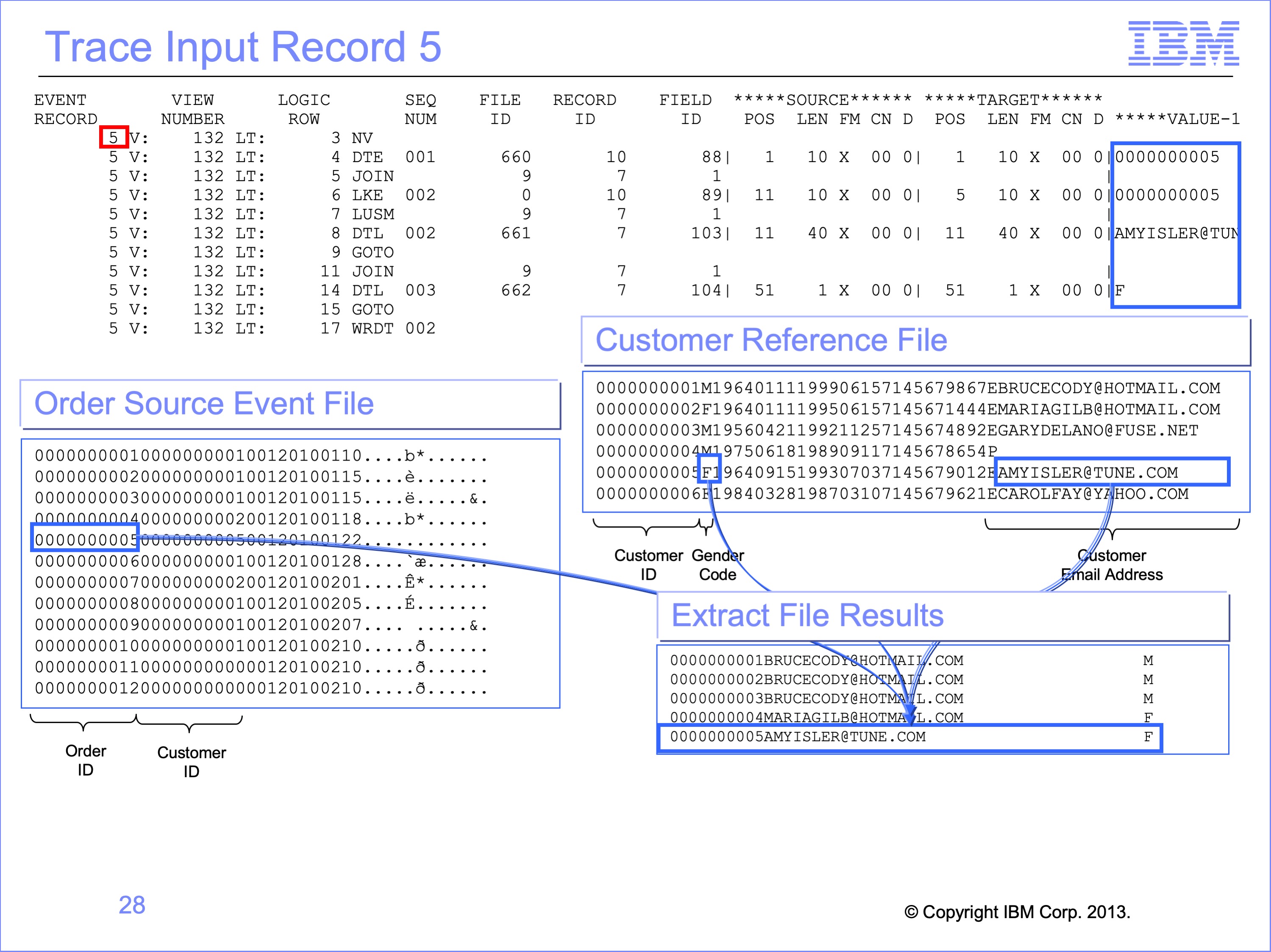
Processing for the next four records continues following the same execution pattern as record number 1. The only changes in the trace are the Event Record number, and the Values on the DTE, LKE, and both DTL functions. The values from the Order and Customer files are moved to the Extract File.
Slide 29
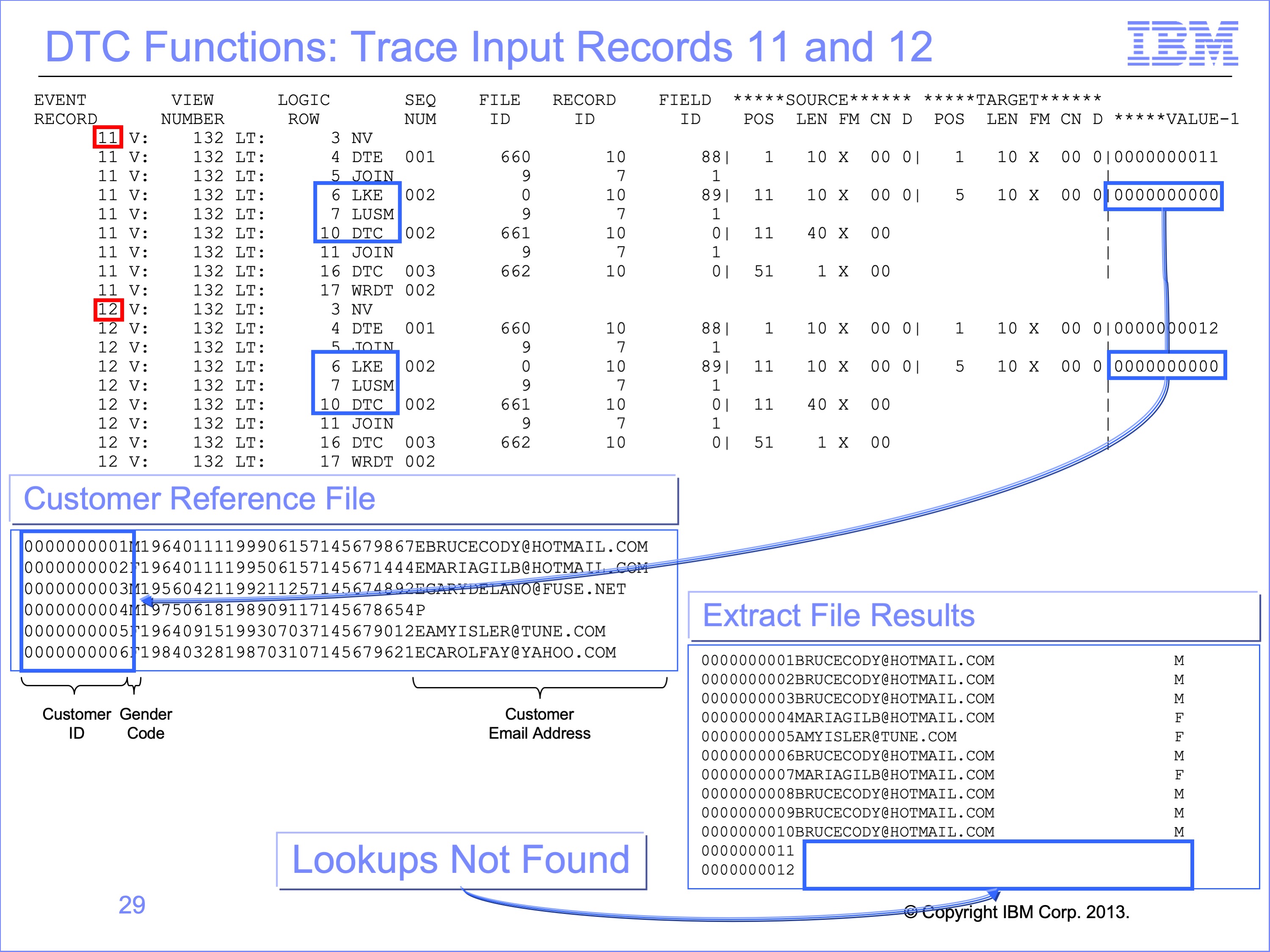
The last two Orders in our example Source Event File do not have corresponding Customer records. Thus on these two records, the first LUSM functions result in Not Found conditions, and branch to the DTC functions to populate the extract record Customer Email Address with the default value of spaces. Likewise, the following Join functions detect that a Not Found occurred on the lookup, and also branch to the DTC functions to populate the extract record with a default space for the Customer Gender code.
We can manually perform the search function by taking the value shown in the LKE function, the “0000000000 “ and searching the Customer Reference File and find there is no Customer record for Customer ID “0000000000”. There can be numerous causes for this, such as non-SAFR issues of mis-matches in the Order and Customer Reference files.
If all lookups fail for a particular reference file it is likely a structural problem. For example, the Join LR may be wrong. Inspecting the RED can highlight this problem. If data displayed in the LKE functions is incorrect, either the Event LR or the path may be incorrect. Partially found lookups may indicate a data issue external to the SAFR configuration.
Slide 30
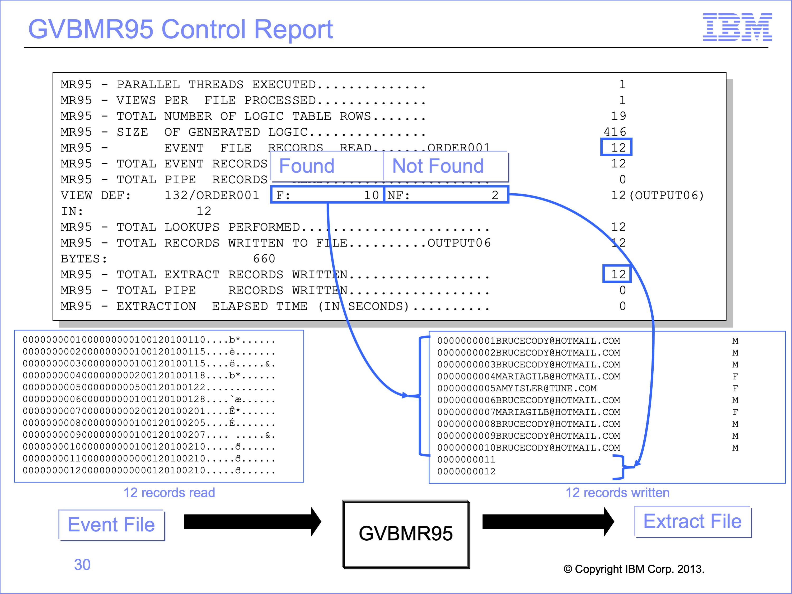
The Extract Engine GVBMR95 control report shows the results of processing. Twelve records were read from the input file, and twelve records written to the output file. For each view against each event file, it reports the total lookups found and not found. The process required 12 total lookups, 10 of which found corresponding records, and 2 which did not.
Note that these counts are the results of LUSM functions, and do not include Join optimizations. If Join optimization had not been performed, the total number of lookups would have been 24, two look up for each extract record written times 12 extract records.
Slide 31
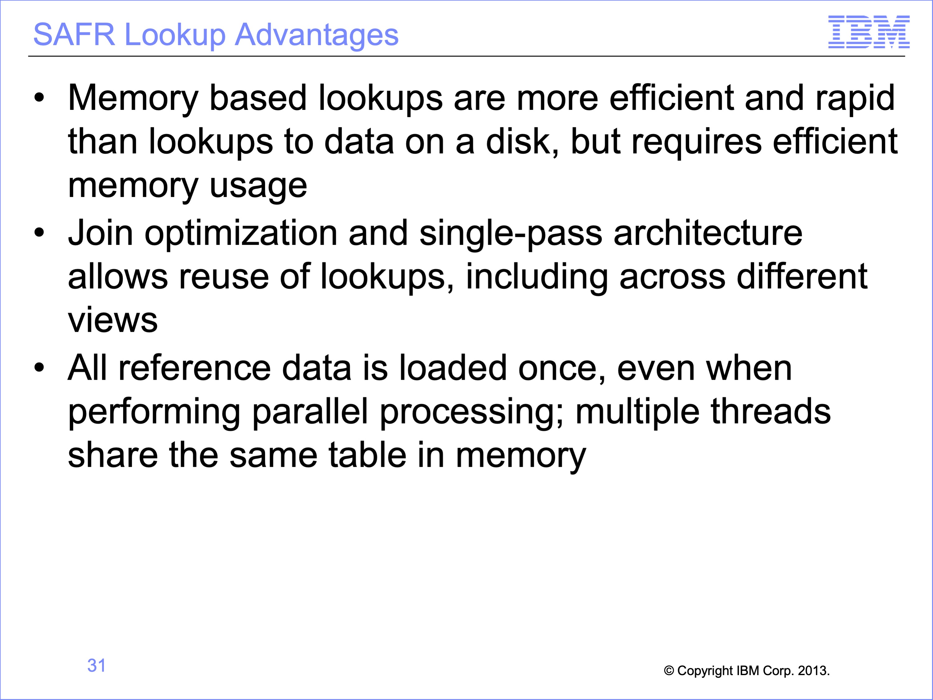
There are many advantages to SAFR’s Lookups processes, allowing it to perform millions of joins or look-ups each CPU second. The following are some reasons for this:
- Memory based lookups are more efficient and rapid than lookups to data on a disk, but requires efficient memory usage
- Join optimization and single-pass architecture allows reuse of lookups, including across different views
- All reference data is loaded once, even when performing parallel processing; multiple threads share the same table in memory
Slide 32
This logic table and module has introduced the following Logic Table Function Code:
- JOIN, Identifies join targets and test for executed Joins
- LKE, builds a look up key using data from the source Event record
- LUSM, binary searches of a in memory reference data table using the Lookup Key
- DTL, moves a looked input field to the output buffer
Slide 33
This module described single step lookup processes. Now that you have completed this module, you should be able to:
- Describe the Join Logic Table
- Describe the advantages of SAFR’s lookup techniques
- Read a Logic Table and Trace with lookups
- Explain the Function Codes used in single step lookups
- Debug a lookup not-found condition
Slide 34
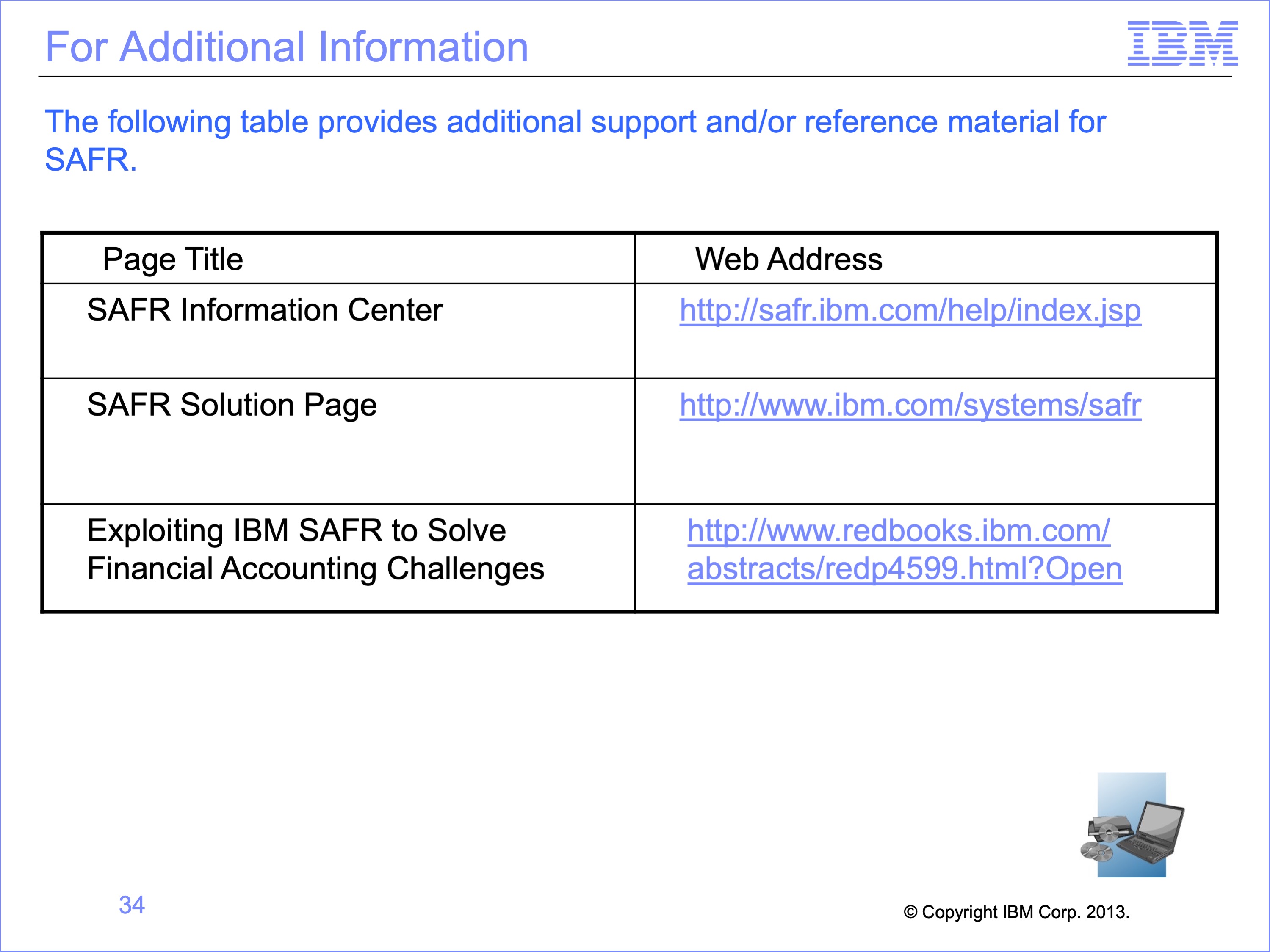
Additional information about SAFR is available at the web addresses shown here. This concludes Module 13, Single Step Lookups
Slide 35