The slides used in the following video are shown below:
Slide 1

Welcome to the advanced training course on IBM Scalable Architecture for Financial Reporting, or SAFR. This is Module 11: Logic Table Introduction and Trace Facilities.
Slide 2

Upon completion of this module, you should be able to:
- Understand the link between the Workbench and the Logic Table
- Describe the purposes of the Logic Table and the Logic Table Trace
- Define a Function Code
- Trace logic through a logic table
- Activate and use the Logic Table Trace
- Debug a SAFR Copy-Input View
Slide 3

The SAFR Workbench allows users to create SAFR views. Once the view is saved and activated in the workbench, it can be used by the Performance Engine, a set of programs run using z/OS JCL. The Performance Engine program GVBMR90 uses the view information in the SAFR Metadata Repository to create a logic table.
The logic table contains the instructions that the SAFR Extract engine (GVBMR95) will use against the input data. As the Extract Engine reads the source data, also called an Event File, the Logic Table instructs it what data to extract to create an output file called the Extract File.
Creating the Logic Table is similar to compiling a program. The view specifications are broken down into individual steps called Logic Table Functions. For example, copying one field in a column from the source file to the output file typically creates at least one logic table function. Logic text for record selection may result in many logic table steps.
Slide 4

Here are examples of main inputs and outputs to the Extract Engine. We’ll explore these in more detail in this module.
The Logic Table is like the source code for a program. By itself, it is static and does not change. The Logic Table Trace is like running a program in a debugger, one instruction at a time. Instead of seeing the program on the screen, the debugger results are printed to a file, one record for each program instruction, showing the impact of each Source or Event File record on the program, and highlighting when and what kind of record is written to the Output or Extract File.
The next few slides will give an overview of the major structures of the Logic Table. An example logic table will then be examined in detail, and later the results of a Logic Table Trace will be shown.
Slide 5

This is a simplified version of a logic table. The compiled instructions from the view are listed as a separate row in the Logic Table. Each row is number sequentially. These rows are used by the GO TO Rows. The GOTO ROW 1 and GOTO ROW2 specify which next Logic Table Row should be executed based upon logic test results.
Most often GO TO Row 1 points to the row to be executed on a TRUE condition, often the next sequential row, and GO TO Row 2 points to the row to be executed on a FALSE condition, often skipping one or more rows.
Slide 6

The Function codes specify what action should be taken. For example, an HD function is the header for the Logic Table, the RENX means Read Next source record, and an NV is the start of a New View. Functions beginning with C compare two values, and functions beginning with W specify writing a record to the Extract File. The ES and EN functions end the logic table.
Slide 7

In this and the next six training modules, you’ll be introduced to all the major Logic Table function codes. To help in remembering what each does, it is useful to remember the following naming rules. Each function code has:
- A two-character function, like LK for Lookup or CF for Compare Field
- Many have one character for the source, such as E for Event File field, L for Lookup, or C for Constant
- Many also have one character specifying the target
Examples include:
- CFEC, which Compares a Field, in this case comparing an Event file field to a Constant;
- LKL, which builds a Lookup Key from a Looked-up value;
- SKE, which builds a Sort Key from an Event file field; or
- DTC, which builds a Data column from a Constant.
Slide 8

The next part of the Logic Table is the Sequence Number. It is used only for certain Logic Table Functions. It can contain either the extract file the record is to be written to, or the column number that required the Logic Table function.
In this example, 1 is the is the extract file ID the Extract record should be written to for the Logic Table Write function WRIN.
Slide 9

The next set of fields are the Logical Record (LR) and Field IDs referenced by a function code. For certain Logic Table functions which require an LR or field, these columns will contain the Workbench ID for the LR or field used. These IDs can be located in the Workbench
In this example the NV New View Logic Table function is using the LR 1264 as the Event File for the view. The CFEC Compare Field Logic Table function is using field 63311 from the same LR as part of its comparison.
Slide 10

The next set of columns specify the source attributes, such as the position of the source field in the event file, its length, its format, the content code if it has one and its decimal places. A full Logic Table report has a duplicate set of these columns for Target or Output attributes as well. Typically these values come from the field assigned to an LR.
- POS is the starting position of the field.
- LEN is the field length.
- FM is Format of the field, such as alphanumeric or packed.
- CN is the date/time format (formerly known as the content code), which specifies the display format of a date or time field.
- D is the number of decimals implicit in a number in the field.
In this example, the field (63311) starts in position 1 and is 9 bytes long. It is a Zoned Decimal format field, with no specific Date/Time Format and no implicit decimals.
Slide 11

The last set of columns vary depending the Logic Table function code. For comparison functions, it contains the type of comparison to be performed, the length to be compared, and the constant to be compared against. In this example the Event File Field is to be compared for an equal condition for nine bytes to the constant of “522349999”.
Other functions codes may display only the constant to be used in the function or other data.
Slide 12

For this module we will use a Copy-Input view, View ID 3261 which simply copies the input records to the output file without reformatting them. In other words, the view copies the entire record from input to output. A copy-input view is used here because it is the simplest of all SAFR views. It does not require any columns or sort fields. We will examine the Logic Table created for this view throughout this module.
A copy-input view has the “Source Record Structure” option selected on the View Properties Tab in the workbench.
If no filtering criteria is coded, all input records will be copied to the output file. Record filtering criteria can be used to select only certain records. In this example, the SelectIf Statement was coded in the logic text. It will result in only records with an input field Legal Entity equaling “522349999” being selected.
Slide 13

The Logic Table shown is for view 3261, our Copy-Input view. It is a complete logic table with only seven Logic Table rows.
The first Logic Table Function in each logic table is an HD or Header Function. This function causes startup functions to be performed, such as allocating memory, and so on.
Each logic table ends with an EN or End Function. The EN function ends all processing.
Slide 14

Each Event File to be read begins with an RENX or Read Next record function. The RENX function brings the next record to be processed into memory. All function codes following the RENX refer to this record. The file ID to be read is identified above the RENX. In this example, the file ID that can be locate in the Workbench for the physical file is 1284.
Each RENX is paired with an ES or End of Source File function. The SAFR extract engine performs all of the functions between these two for every record within the file. In other words, when the Extract Engine reaches the ES function, it loops back to the RENX to read the next record in the Source or Event file.
Slide 15
Slide 1

Each View begins with an NV or New View function. The NV function tests if the view has been disabled, for example if an extract limit has been reached for the view. If so, all logic table functions for the view are skipped and the next view is processed. The NV is preceded by the View ID, in this case view number 3261
Each NV is paired with a WR Write function of one type or other. A copy-input view ends with a WRIN Write Input record function. The sequence number in WR functions indicates which extract file the records are written to.
Slide 16

In between the NV and WR functions are optional functions to perform the logic required by the view. Most Logic Tables contain at least five to ten logic table rows for logic.
Our very simple copy-input view, though contains only one user-specified function, the CFEC function, a Compare Field, Event file field to Constant. The CFEC row was created because the view contains a general selection logic text SELECTIF function. CF stands for Compare Field.
The “E” in CFEC means event file field, a field on the input file. The Event File field—the field to be tested—is the Legal_Entity field from the LR 1264 field ID 63311. That field is at position 1, for a length of 9, and zoned numeric format (FM=3) with no decimal places.
The second C in CFEC stands for a constant. The type of comparison is an equal test (CMP = 001) to the constant value of “522349999” which has a length of 9 bytes.
Slide 17

The CFEC function uses the GO TO Rows to indicate what should be done based upon the test. If the current event record constant comparisons proves true, the row in the GOTO ROW1 is executed. If the comparison is false, the GOTO ROW2 will be executed.
In our example, if the Legal_Entity field contains a value of 52234999, execution continues at Row 5, the WRIN function which writes the input record. If Legal_Entity contains another value, the comparison proves false, and execution continues at GOTO Row 6, the ES row. The ES function causes a loop to the RENX function which causes the next event record to be read.
Slide 18

As explained earlier, the Logic Table is like a program listing, but it does not show how the program executes over time. A program in a debugger, showing which logic paths are executed, is like the Logic Table Trace.
In the EXTRACT phase, the MR95 TRACE function writes each executed row of the logic table to a report to aid you in debugging a view. The TRACE function can be selected and configured in MR95PARM, the MR95 parameter file. Trace shows how each record in the input file is processed through the logic of the Logic Table, one instruction at a time.
The MR95 trace can become very large very quickly. Imagine the input file contains 1 million records, and the logic table has 1000 rows. The total trace output could be 1 billion rows of printed data!
Using the MR95 trace can also significantly impact performance. It should be used with care. Reducing the input Event File size is the most effective way to control the performance of trace processing.
Slide 19

When the Trace parameter is set to “Y”, additional parameters are available to control what is traced. If, for example, the file sizes cannot be reduced, these parameters can be used to reduce the trace output or isolate specific records or problems.
The following are the more detailed trace control parameters:
- The TRACEINPUT parameter will print in dump format the entire source record at read time.
- The VIEW parameter will trace only for the specific view.
- The LTFUNC parameter will trace only a specific logic table function, like a CFEC function.
- The DDNAME will trace only that input file.
- FROMREC and THRUREC will trace from a specific record to a specific record in the input file.
- Similarly FROMLTROW and THRULTROW will trace only specific logic table rows.
- LTABEND will cause MR95 to produce a dump for debugging if it executes a specific logic table row.
- And MSGABEND will cause MR95 to abend if it produces a specific error number, like an 0C7 data exception.
- Lastly, the VPOS, VLEN, and VALUE parameters trace only when the data at position for length on the source record is equal to a specific value.
Although these functions are very powerful, they significantly increase GVBMR95 processing time even if they suppress trace records from being printed to the output file. Therefore, reducing the file size is much more efficient if possible. We’ll show examples of how to use them to find and fix problems in more detail in Module 15, Lookups using Constants and Symbolics
Slide 20

This is the logic table trace output. The first column contains the EVENT DDName. This is the DD Name of the Event file, which contains the source data. If the Extract Engine is performing parallel processing, each row may show data from a different input file.
The Event Record column shows the input record number from that event file. Because each input record is executed by numerous logic table rows, record 1, for example, shows multiple times in this output.
The View and Logic Row columns show which logic table row execution is occurring. The row number is the sequential number row—the first column—of the logic table.
The Value 1 and Value 2 columns show the data used in things like comparisons. Value 1 typically shows the data from a file or a lookup, the E of a CFEC or L of a CFLC. Value 2 often shows a constant value from logic text, the second C in both these functions.
Not shown in this example are the source and target attribute columns, which are similar to those in the logic table, containing the starting position, length, and format of the fields.
Slide 21

This logic table trace shows what rows of the logic table were processed against each input record. In this example, event record 1 from the EVENT file was processed against NV, Logic Table Row number 3. Record one is then processed against Logic Table row 4.
Later, after completing the loop for Record 1, Record 2 of the input file is processed against NV function Logic Table row 3. Some rows are not shown in the report, like the HD, RENX, ES and EN rows.
Slide 22

When record 1 is processed against the CFEC function on logic table row 4, Value 1 shows the value in the event record—the “E” in CFEC—and Value 2 shows the constant in the
logic text. The two values are equal. So the next row to be executed is the true row, or the GOTO 5 row.
Execution continues at logic table row 5, the WRIN row which copies the event record to the output file.
Slide 23

When record 2 is processed against the CFEC function on logic table row 4, the same pattern is repeated. Because the value in the file and the constant are equal, processing continues with Row 5 of the Logic Table, which writes the input record to the output file.
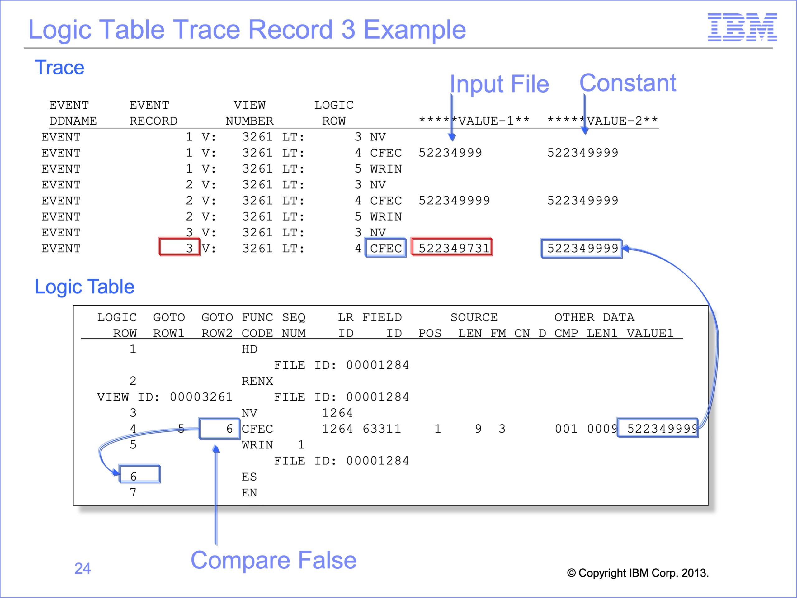
Slide 24

On the third record, the CFEC comparison shows that the value in the event file record, ending in 731, is not equal to the constant ending in 999. Thus the program jumps to the GOTO 2 row or false row 6. Since this is the last record in the event file, the program ends at the ES row of the logic table. The record is not written to the output file.
Slide 25

To recap, this logic table trace contained the following functions:
- CFEC, which compares a constant from the Logic Table to a field in the input file
- WRIN, which writes the input record to the extract file
The Logic Table Trace does not show
- HD, Header function which begins each Logic Table
- RENX, which moves a record from the input Event File to the computer memory
- ES, End of String, which is the end of logic for a specific event file
- EN, End of Logic Table, the last function in the Logic Table.
The function provided by this view is very simple. However, because SAFR generates machine code, it is even more efficient than is available in COBOL. The CFEC function requires two single machine instructions. The assembler instructions generated from the COBOL IF statement are typically many more. The same is true of the WRIN and RENX instructions. This gives SAFR a significant performance advantage.
Slide 26

This is a list of the most common Logic Table Functions and which training module these will be discussed in, for reference.
Slide 27

This module provided an introduction to the Logic Table and the Trace. Now that you have completed this module, you should be able to:
- Understand the link between the Workbench and the Logic Table
- Describe the purposes of the Logic Table and the Logic Table Trace
- Define a Function Code
- Trace logic through a logic table
- Activate and use the Logic Table Trace
- Debug a SAFR Copy-Input View
Slide 28

Additional information about SAFR is available at the web addresses shown here. This concludes Module 11: Logic Table Introduction and Trace Facilities
Slide 29