The following slides are used in this on-line video :
Slide 1

Welcome to the training course on IBM Scalable Architecture for Financial Reporting, or SAFR. This is Module 1: Introduction to SAFR Views.
Slide 2
This module provides you with a broad overview of the SAFR product and the basics of its graphical user interface. By the end of this training, you should be able to:
- Identify the two major software components of the SAFR product
- Identify the major types of SAFR metadata
- Navigate the SAFR Workbench, and
- Create a simple view.
Slide 3
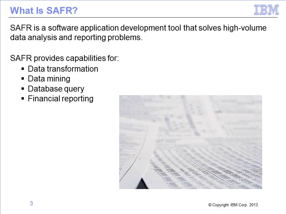
SAFR is a software application development tool that solves high-volume data analysis and reporting problems. SAFR provides capabilities for data transformation, data mining, database query, and financial reporting.
Slide 4
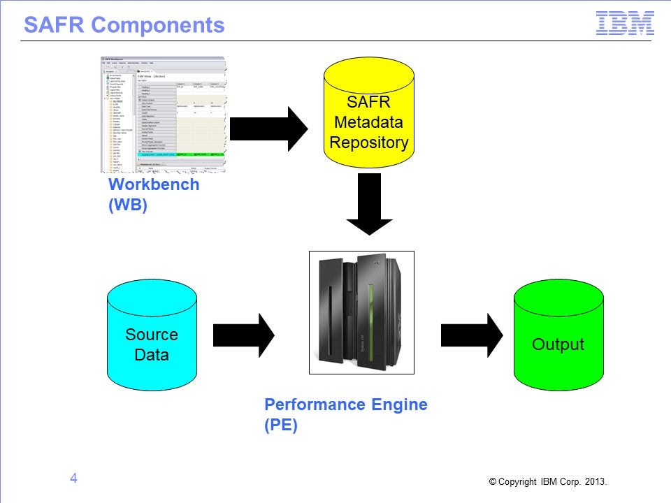
SAFR consists of two software components: the PC-based Workbench and the mainframe-based batch process known as the Performance Engine. Developers use the Workbench to build applications that are stored in a metadata repository in an IBM® DB2® database. These applications are then run by the Performance Engine, which reads data from source files or databases, transforms it, and writes it to output files.
Slide 5
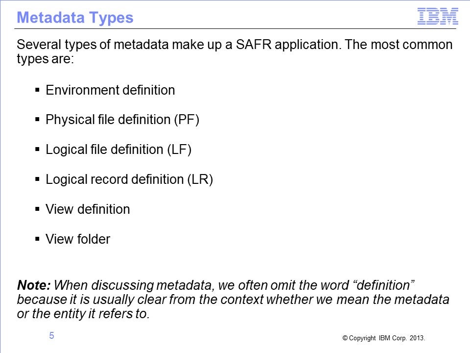
Several types of metadata make up a SAFR application. The most common are the environment definition, the physical file definition (or PF), the logical file definition (or LF), the logical record definition (or LR), the view definition, and the view folder.
Note that, when discussing SAFR metadata, we often omit the word “definition” because it is usually clear from the context whether we mean the metadata or the entity it refers to.
Slide 6
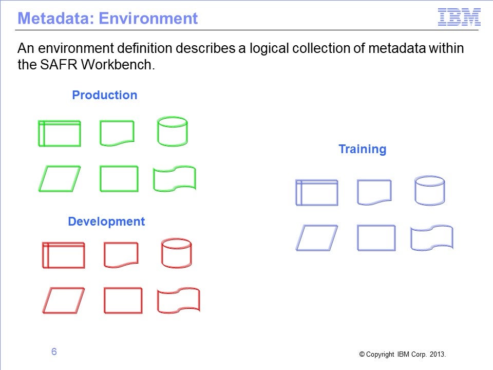
An environment definition describes a logical collection of metadata within the SAFR Workbench. Typical types of environments include development, production, or training environments. Access to an environment can be restricted to a certain set of users.
Slide 7
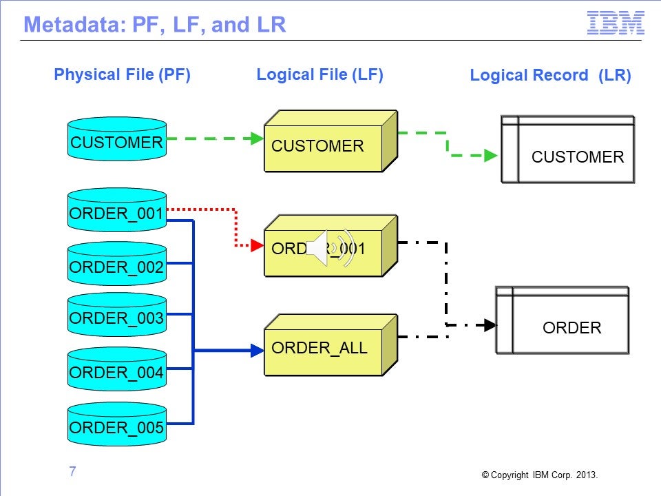
A physical file definition, or PF, describes a data source. Examples include customer or order files. A logical file definition, or LF, describes a collection of one or more physical files. A logical record definition, or LR, describes a record layout. In COBOL programs, record layouts are often found in copybooks. In relational databases, they are found in table definitions.
Some examples of these metadata types are shown here.
- A logical record for a customer is used to map data to a customer logical file. The customer logical file refers to data in a customer physical file.
- An order logical record is used to map data from a logical file named ORDER_001, which refers to data in a single physical file named ORDER_001.
- The order logical record can also be used to map data from a logical file named ORDER_ALL. ORDER ALL refers to a collection of order physical files.
Slide 8
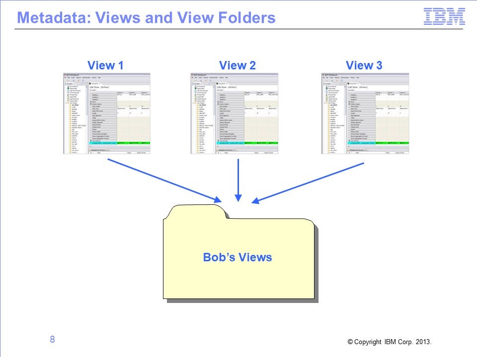
A view definition describes a data transformation. It is analogous to a program or a query. Views are the basic units of work that are performed by the Performance Engine.
Views are often grouped together into view folders for ease of maintenance. View folders are often named for a particular developer or function. Security can be applied to view folders to prevent unauthorized access.
Slide 9
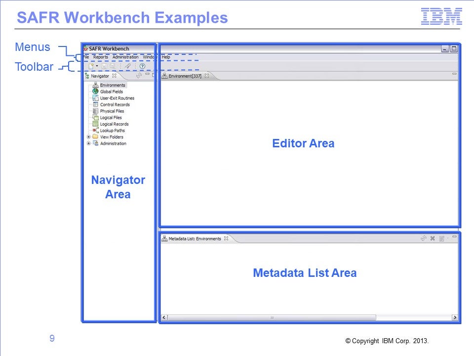
The SAFR Workbench is used to add, change, and delete SAFR metadata. It contains a menu and toolbar, and consists of multiple display areas, or frames.
- The Navigator area displays the types of metadata available.
- The Metadata List area displays a list of items for the selected metadata type.
- And the Editor area is the part of the screen where you modify metadata items.
Slide 10
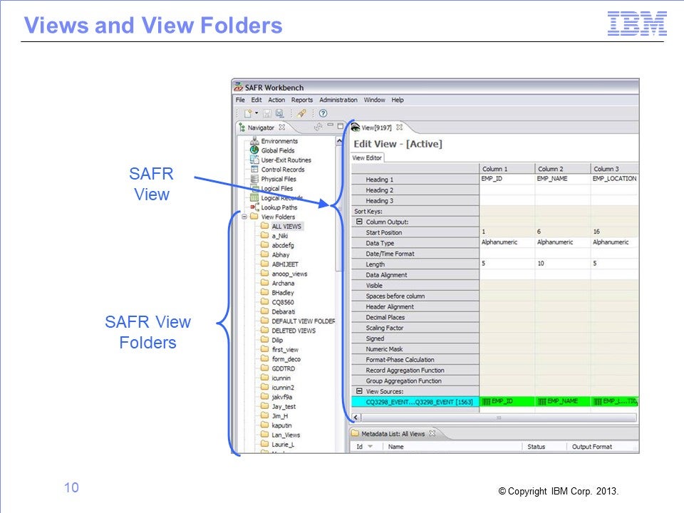
- By expanding the View Folders item in the Navigator area, you can see a list of all view folders.
- The contents of the selected folder are displayed in the Metadata List area.
- From there, you can select a view for editing and the view will be displayed in the Editor area.
Slide 11
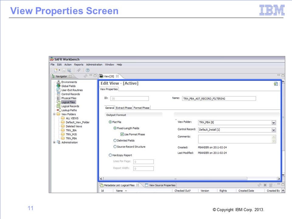
View information is displayed on two separate screens:
- The View Editor screen, where you can define specific data transformations.
- The View Properties screen, where you can modify information that applies to the whole view.
Slide 12
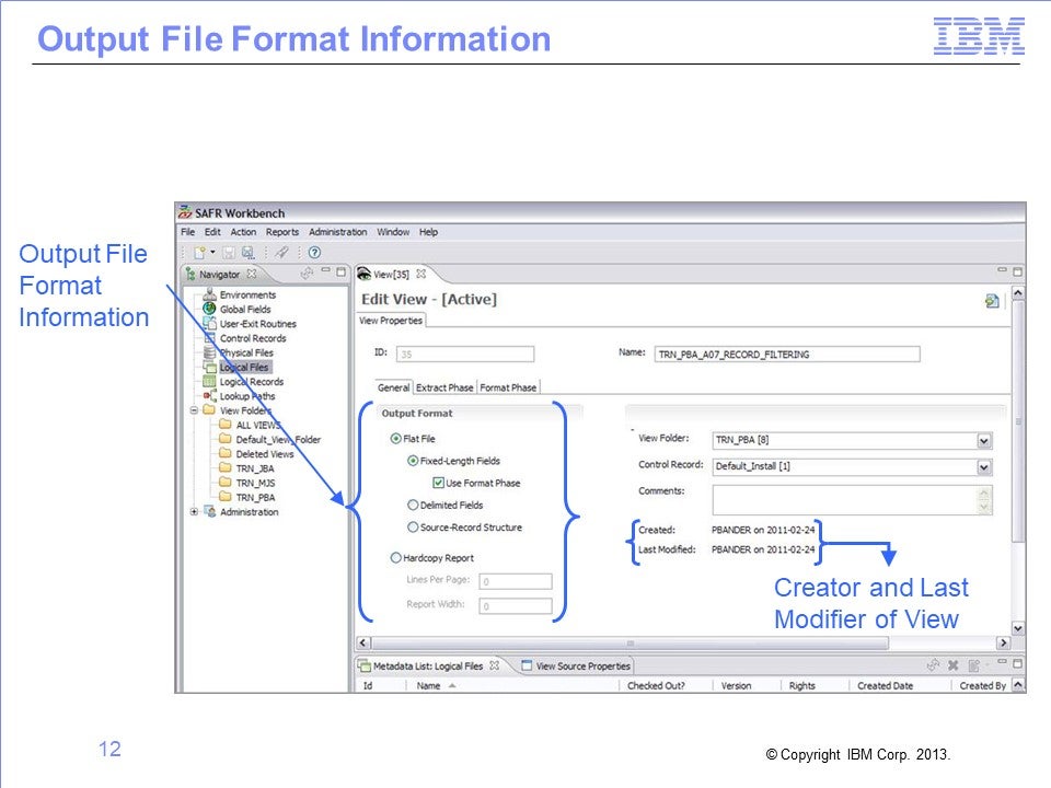
You use the General tab on the View Properties screen to specify the output format – flat file or hardcopy report – and other related information.
This tab also displays information about when the view was created and last modified and by whom.
Slide 13
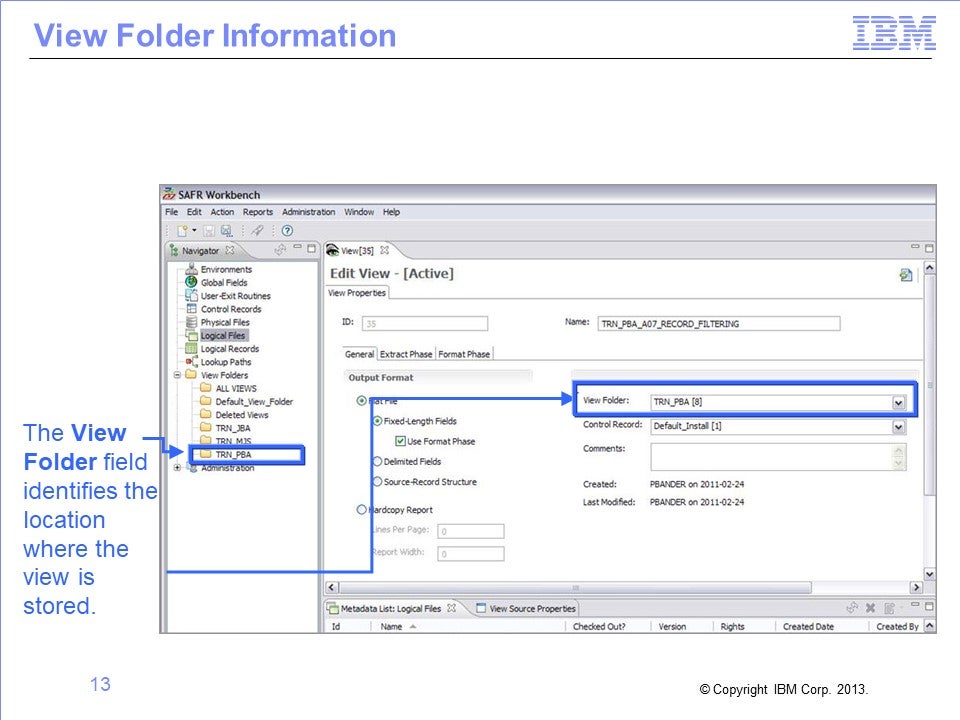
In addition, the General tab displays the name of the view folder where the view is stored.
Slide 14
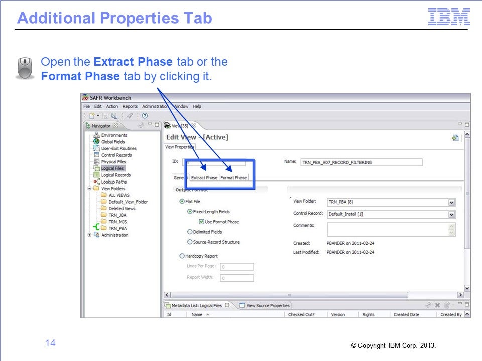
You can access advanced features on the Extract Phase tab and the Format Phase tab. You can open these tabs by single-clicking them.
Slide 15
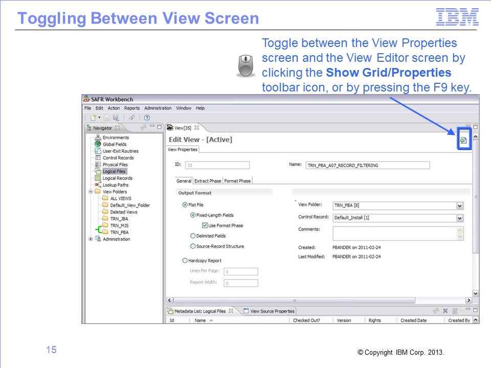
You can toggle back and forth between the View Properties screen and the View Editor screen by clicking the first icon in the Editor area toolbar, or by pressing the F9 key.
Slide 16
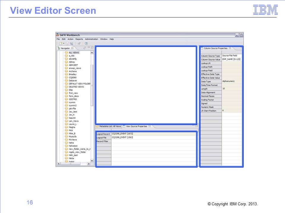
In View Editor mode, the Workbench displays several frames of view information.
Slide 17
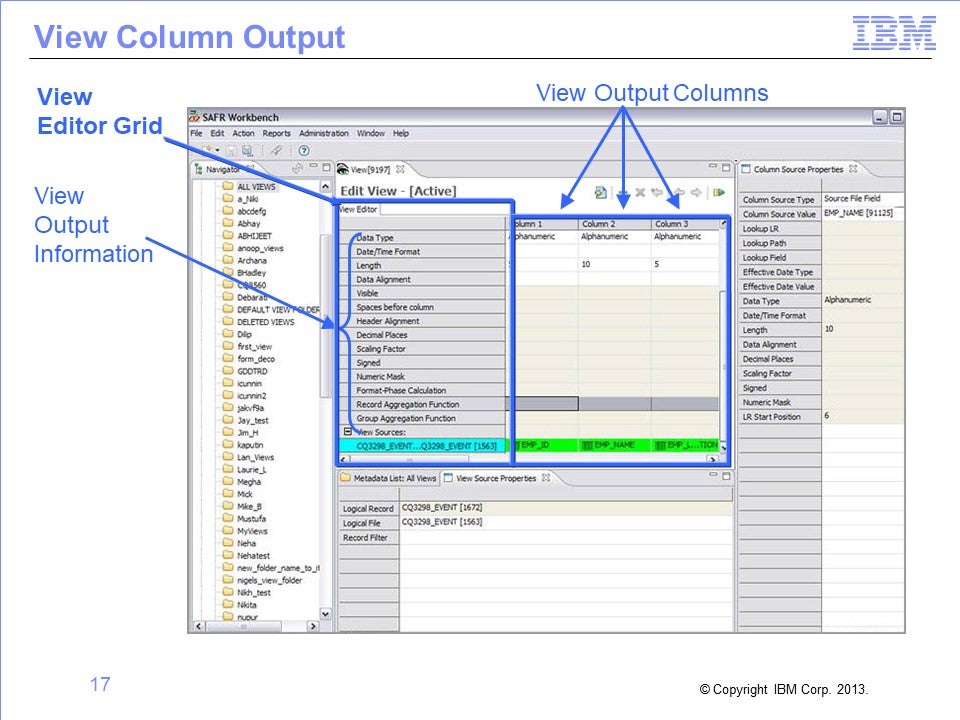
The View Editor grid displays the characteristics of view output columns. These characteristics include the data type, the length, and the alignment, such as left, right, or center.
Slide 18
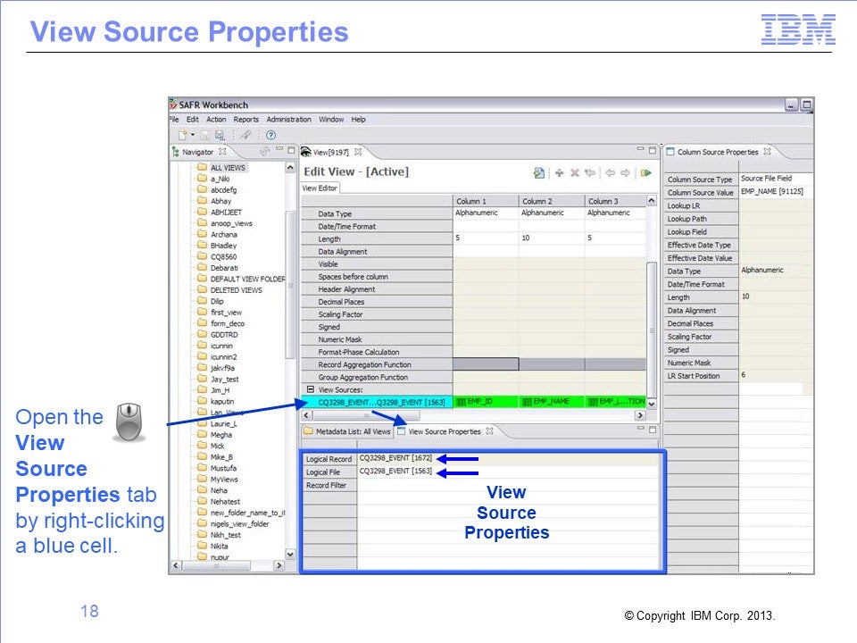
You can display information about the data source for the view by right-clicking a blue cell in the View Editor grid. This information includes the logical record and the logical file.
Slide 19
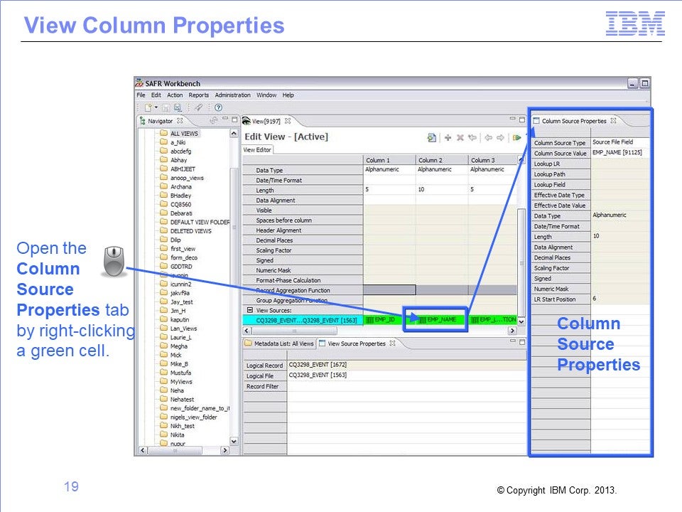
To open a frame showing the column source properties, you right-click a green cell. The source of a column’s data can be a field in the source file, a constant, a lookup value, or the result of a formula.
Slide 20
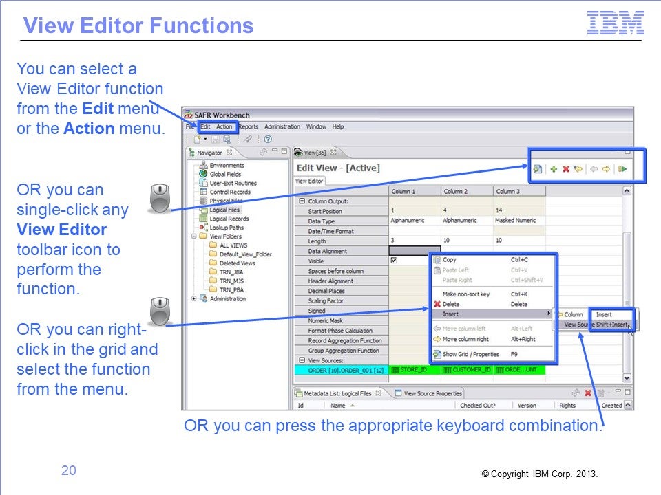
The View Editor incorporates several functions, such as inserting a column or activating a view. You can run a View Editor function in several ways:
- Select it from the Edit menu or the Action menu for the Workbench
- Left-click the function icon on the View Editor toolbar
- Right-click in the View Editor grid and select the function from the pop-up menu
- Or press the appropriate key combination, which is noted on the Workbench menu and the pop-up menu.
Choose whichever technique you prefer.
Slide 21
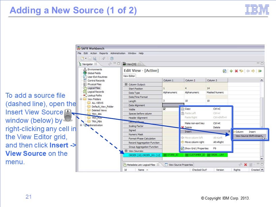
To add a new view source, you right-click on the grid to display the pop-up menu, and then select Insert and View Source.
Slide 22
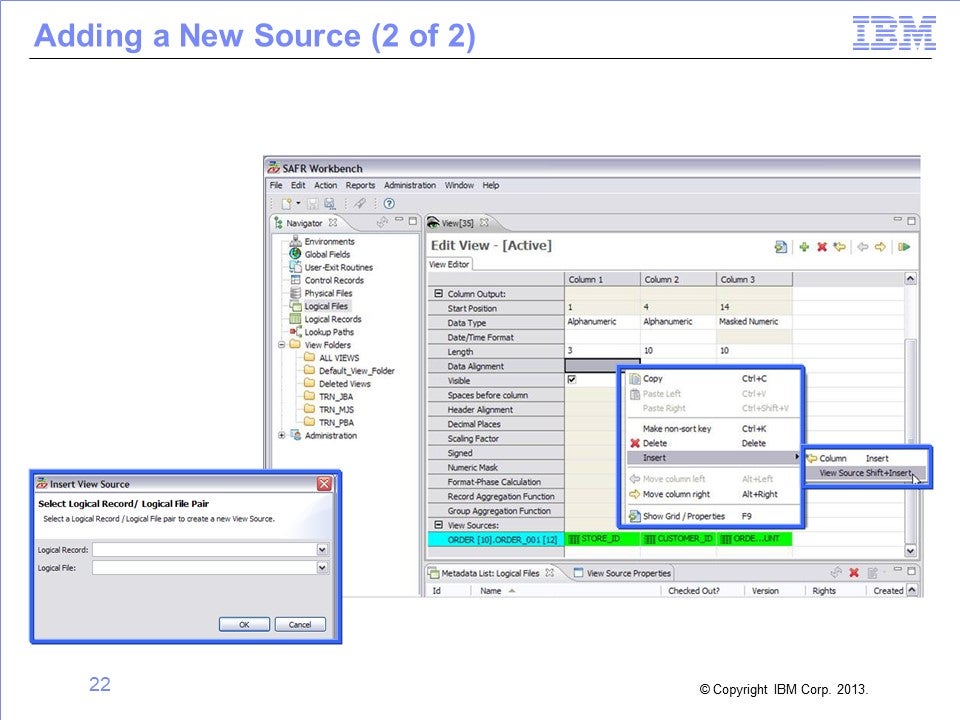
The Insert View Source window opens. You can select from a list of data sources in the window.
Slide 23
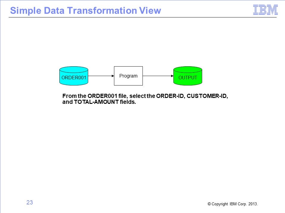
Now let’s take what you’ve learned and create your own view. The following example is a simple data transformation, reading data from the ORDER001 file and writing out only the Order ID, Customer ID, and Total Amount fields.
Slide 24
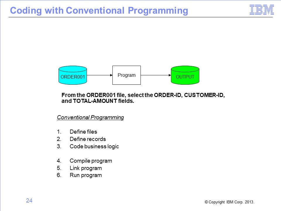
If we were to code a conventional program, we would:
- Define the file attributes
- Define the record layouts
- Code the business logic
- Compile the program
- Link the program and
- Run the program
Slide 25

With the SAFR tool, the first three steps are performed in the Workbench and the last three are performed for you by the Performance Engine.
Slide 26
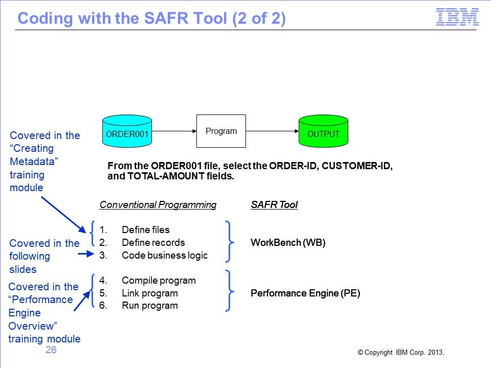
Defining files and records will be covered in the SAFR training module entitled “Creating Metadata.” The Performance Engine will be introduced in the “Performance Engine Overview” module. The topic of coding business logic will be introduced in the next few slides.
Slide 27
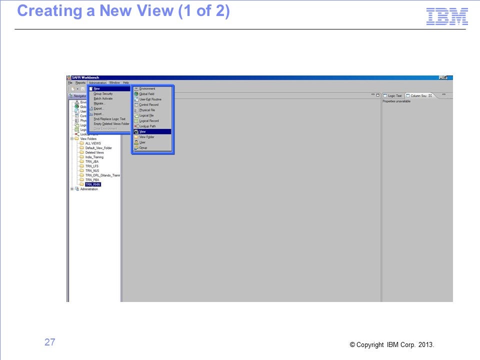
In the example described in the following slides, metadata has been pre-populated in the Workbench for ease of instruction.
To create a new view, click the Administration menu, select New and then select View.
Slide 28
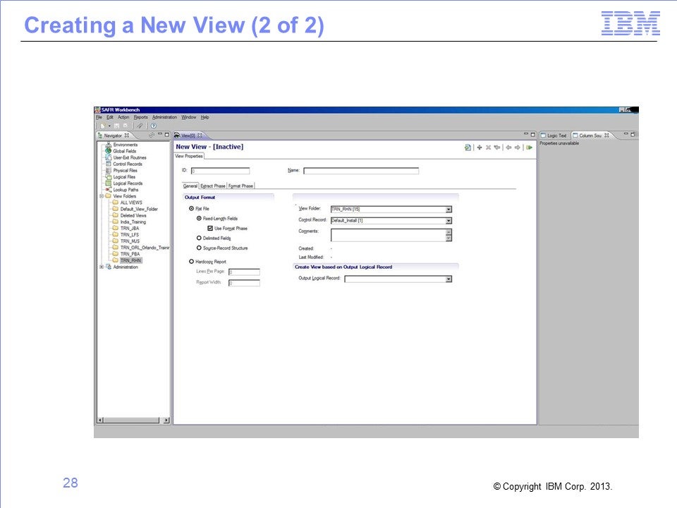
The View Properties tab opens.
Slide 29
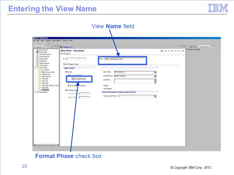
Enter a descriptive name for the view, such as “Simple_Transformation_View.” Note that embedded spaces are not allowed in names, so you must use underscores to separate words. Next, clear the Format Phase check box; this feature is not needed for this simple view.
Slide 30
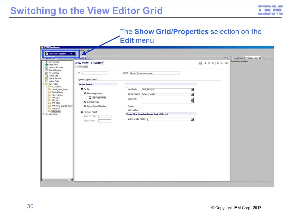
To display the View Editor Grid, select Show Grid or Properties, from the Edit menu (Alternatively, you can click the toolbar icon or press the F9 key).
Slide 31
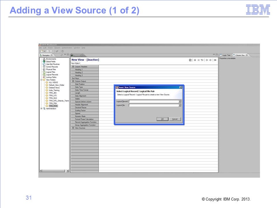
From the Edit menu, select Insert, and then select View Source (Alternatively, you can right-click and select Insert and then select View Source from the pop-up menu, or you can press the Shift key and the Insert key). The Insert View Source window opens.
Slide 32
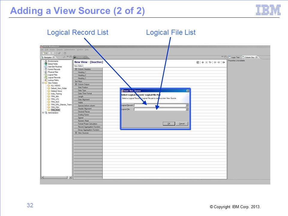
From the Logical Record list, select ORDER. Then, from the Logical File list, select ORDER_001.
Slide 33
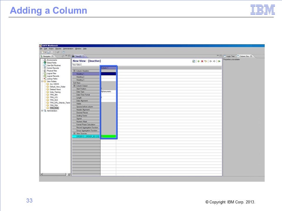
From the Edit menu, select Add Column (Alternatively, you can click the plus sign icon on the toolbar or press Alt and the Insert key). A new column is added to the grid.
Slide 34
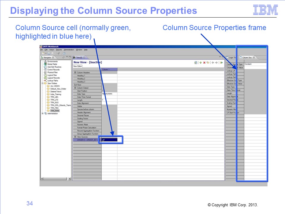
Click the green cell. The Column Source Properties frame opens on the right.
Slide 35
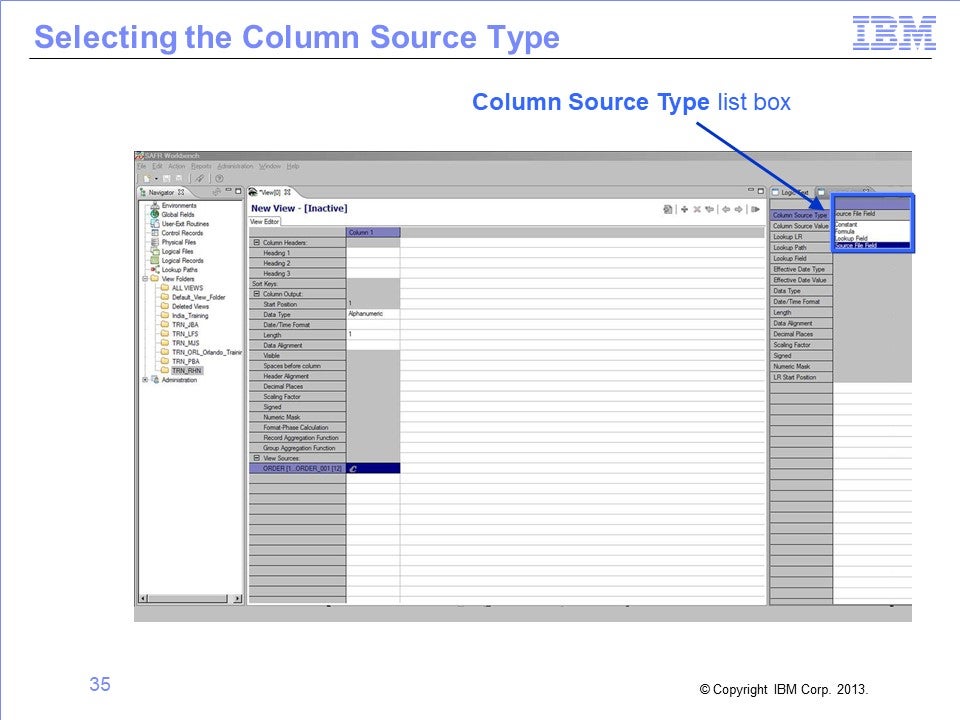
In the Column Source Type field, click the list box and select Source File Field.
Slide 36
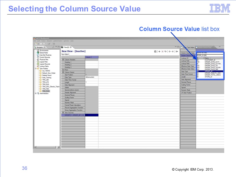
In the Column Source Value field, click the list box and select ORDER_ID.
Slide 37
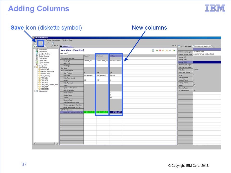
Repeat the previous steps to add columns for Customer ID and Order Total Amount. Then save the view by selecting Save from the File menu, or by clicking the Save icon in the Workbench toolbar, or by pressing Control and S.
Slide 38
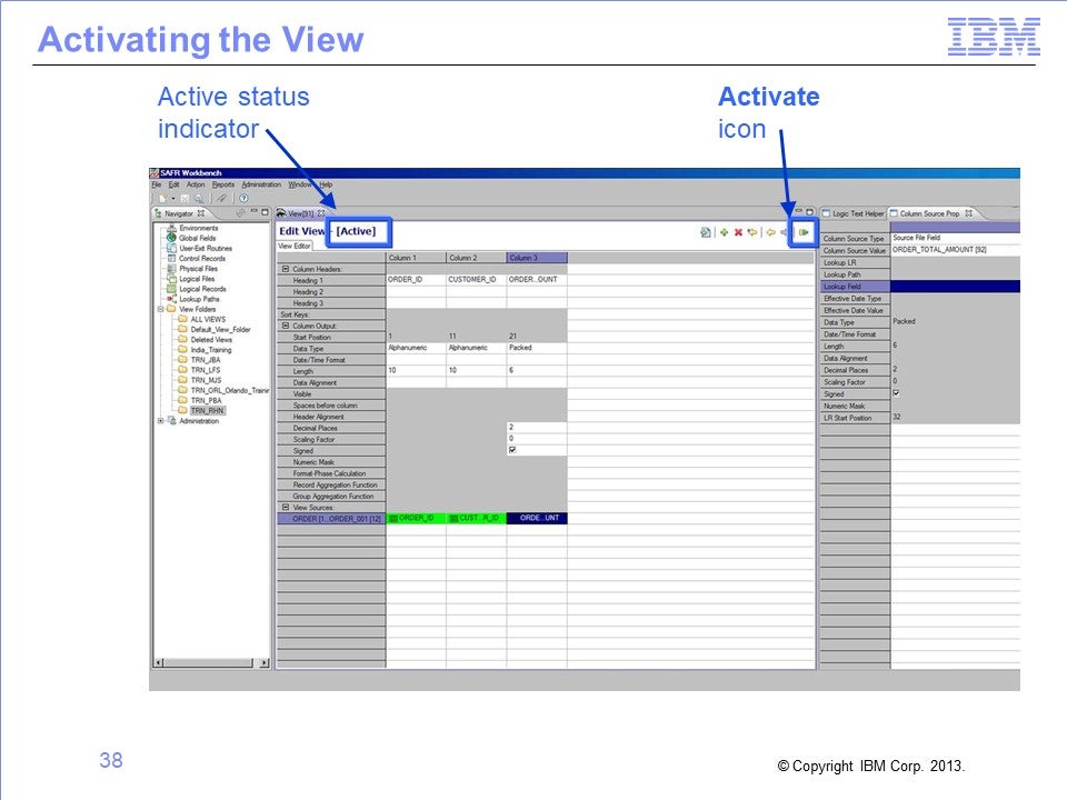
To activate the view, use any of these methods:
- Select Activate from the Action menu
- Press the Activate icon on the View Editor toolbar
- Press F5.
The view title bar now displays the word “active”. Save the view again to preserve this active state. The view is now ready to be run.
Slide 39
This module provided an overview of SAFR. Now that you have completed this module, you should be able to:
- Identify the two major software components of the SAFR product
- Identify the major types of SAFR metadata
- Navigate the SAFR Workbench and
- Create a simple view